This is the 29th post in a series of Nikon D850 tests. The series starts here.
In the preceding three posts, I looked at the on-axis sharpness and longitudinal chromatic aberration (LoCA) of the Sigma 135 mm f/1.8 ART, 85 mm f/1.4 ART, and 105 mm f/2.8 macro lenses on the Nikon D850. Now I’ll do the same test with the Sigma 35 mm f/1.4 ART lens.
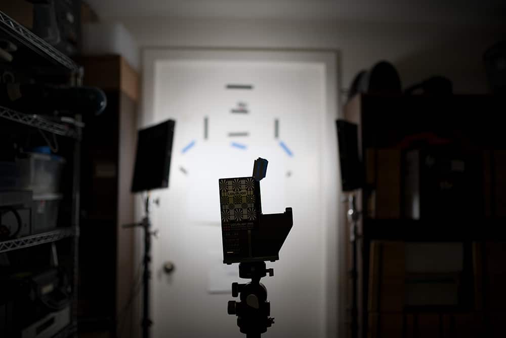
The target is a backlit razor blade:
The test protocol:
- ISO 64
- Focus shift, silent shutter option
- 40 steps
- Minimum step size (1)
- Target distance, 1 meter
- Aperture exposure mode
- Wescott LED panels set to 5500 K.
- Gitzo legs
- Arca Swiss C1 head
- Vinyl tile flooring over 6 inches of concrete on grade
- Fast Raw Viewer to discard the really out of focus images
- dcraw in document mode to get raw planes
- MTF Mapper to compute MTF50
- Matlab to automate the above
- Excel to graphs the results
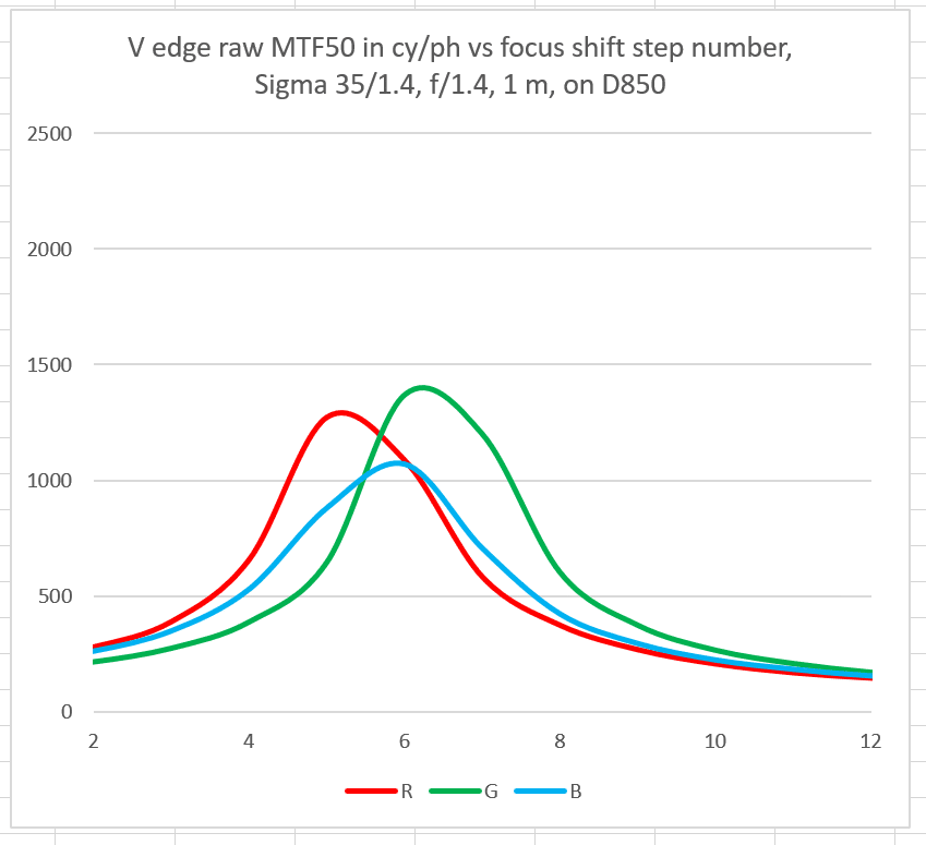
Here are the results wide open:
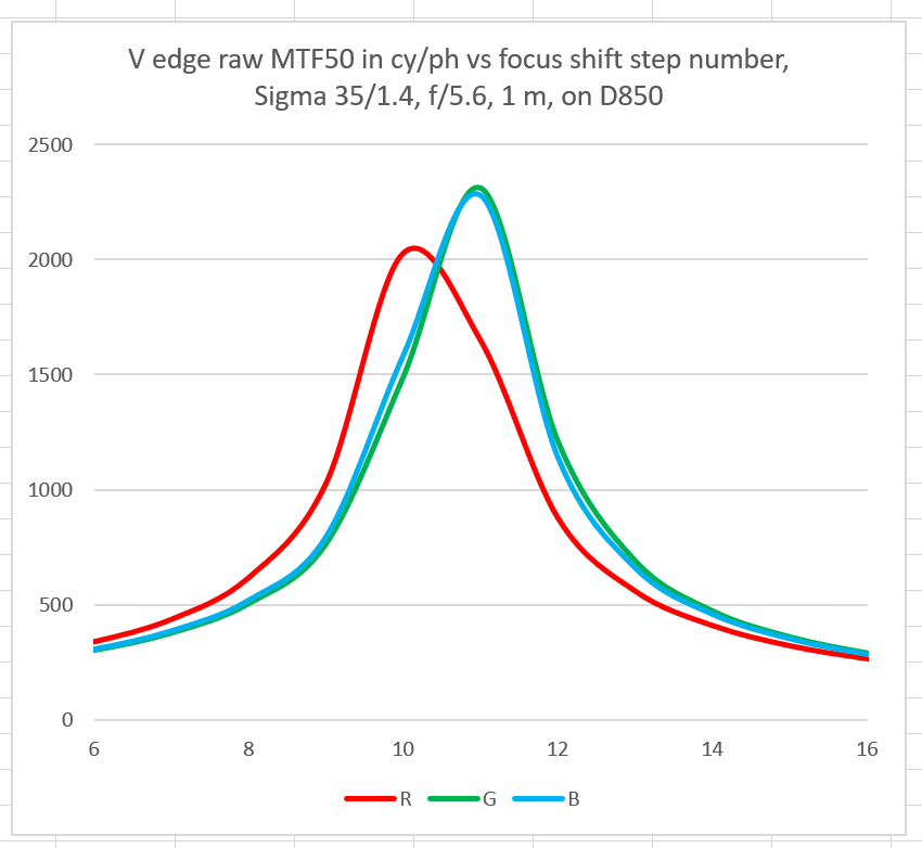
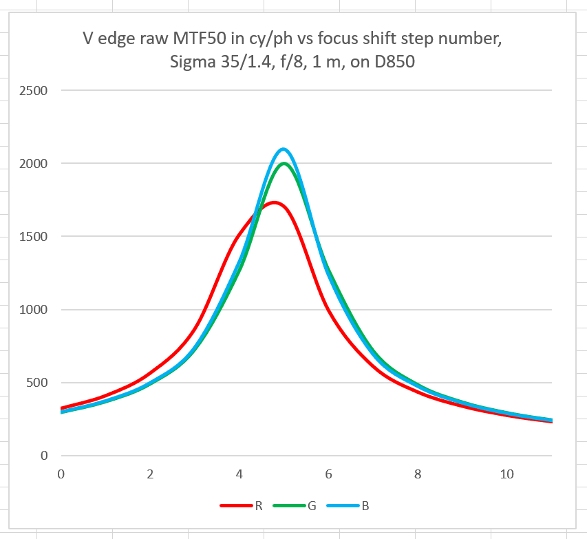
The vertical axis is MTF50, measured in cycles per picture height (cy/ph). The shot taken with the lens focused to the closest position is on the left. There are 11 exposures plotted. There is no way to know the focused distance for these exposures. I used the minimum step size for the Focus Shift Shooting feature, which is too large to reliably catch the actual peaks, but it’s not that bad.
Not bad for f/1.4. There is quite a bit of longitudinal chromatic aberration (LoCA).
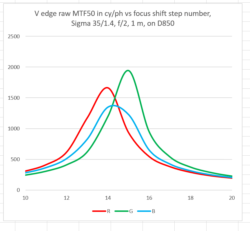
The sharpness comes up a lot at f/2.
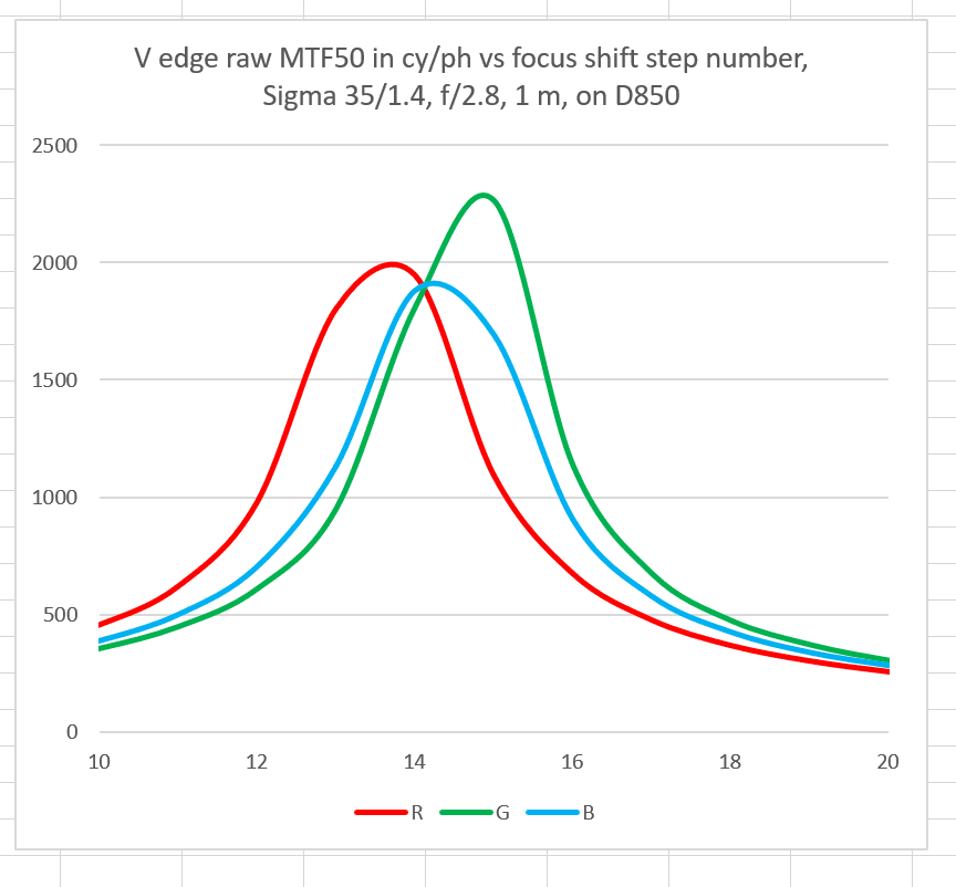
At f/2.8, it’s starting to get good, but it gets better.
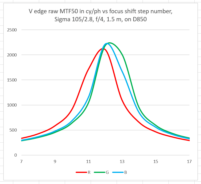
Ignore the title on the above graph. It’s really 35/1.4 at f/4 ,and it’s really 1 meter.
At f/4, this is a seriously sharp lens, and the LoCA is well under control.
Sharpness is falling off at f/5.6, but it’s still excellent.
At f/8, the LoCA is all masked out by the DOF, and it’s still darned sharp.
On-axis, this is an excellent lens.
Jack Hogan says
Hi Jim, nice series! Looking at the distorted curves in it I can’t help but wonder whether it would be worthwhile to use interpolation that better approximates actual physical performance (as measured with your rail protocol) or simply not to interpolate at all.
Jack
JimK says
Good point. What do you think about fitting a Gaussian PDF?
Y = normpdf(X,mu,sigma)
Frans van den Bergh says
I have obtained good results by fitting a rational polynomial to the MTF50 vs distance data. My objective was to find the most stable fit, such that repeated photos of the same set-up would yield the smallest spread in the estimated peak distance of the MTF50 vs distance curve.
In particular, I start by fitting (a_0 + a_1*x + a_2*x^2 + a_3*x^3 + a_4*x^4) / (b_0 + b_1*x + b_2*x^2). If this turns out to have a pole inside the range interval, I reduce the order of the numerator polynomial.
So far this scheme has been working quite well.
-F
Jack Hogan says
That’d be a good start. It would probably be worth limiting the fit to just a few samples on either side of the peak.
Brandon Dube says
There’s a closed analytic form for the diffraction MTF through focus — I forget exactly what it is at the moment, but it’s sinc or jinc like. Peak with lobes and all that. Spherical pushes more energy into the lobes and adds a linear term, which you can think of as putting some moment/momentum into the curve.
IDK how MTF50 will “react.”
Your curves look, more or less, like gaussians or supergaussians, with some of that spherical related moment to them.
Richard Scobie says
Hi Jim,
Minor nit – you’ve mis-labelled the f4 chart as “Sigma 105/2.8”.
Regards,
Richard
JimK says
Thanks. I’ve written text below the image calling attention to the error.
Michael Demeyer says
Jim,
Would be interesting to run a rail set to see how the focus-shift actually shifts the focus of the lens, particularly what factors it considers in selecting the focus steps. You mention the steps being more widely spaced as you stop down, which seems evident from the left-ward shift in the curves overall. Does it also consider focal length, for example?
Michael