Leica M240 banding, part 3

I’m beginning to get a handle on what’s going on with the M240 shadow behavior vs camera ISO setting.

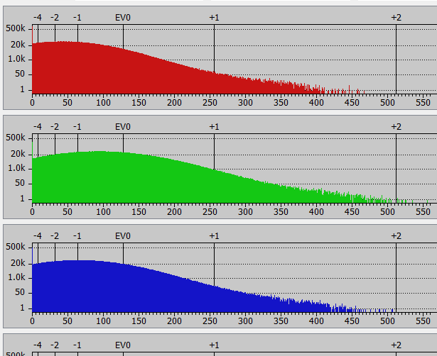
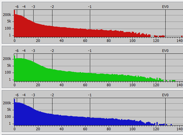
Here’s a series like that in the preceding post, but one stop more exposure, placing the average of the image values at ISO 3200 about 7 stops below full scale. The light is falling on the projection screen from the left, so you can see how the image behaves as the exposure decreases by scanning from left to right. I’ve put the hisotgrams of the raw files below the converted images so you can see what’s happening.

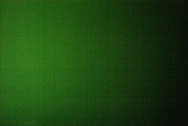
ISO 3200:

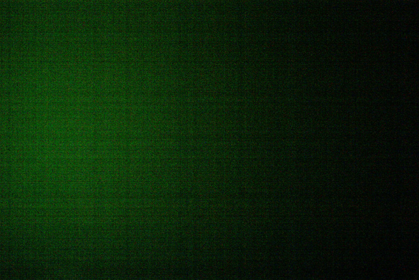
ISO 1600, with a one stop push in ACR:

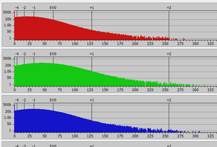
ISO 800, with a 2-stop push in ACR:

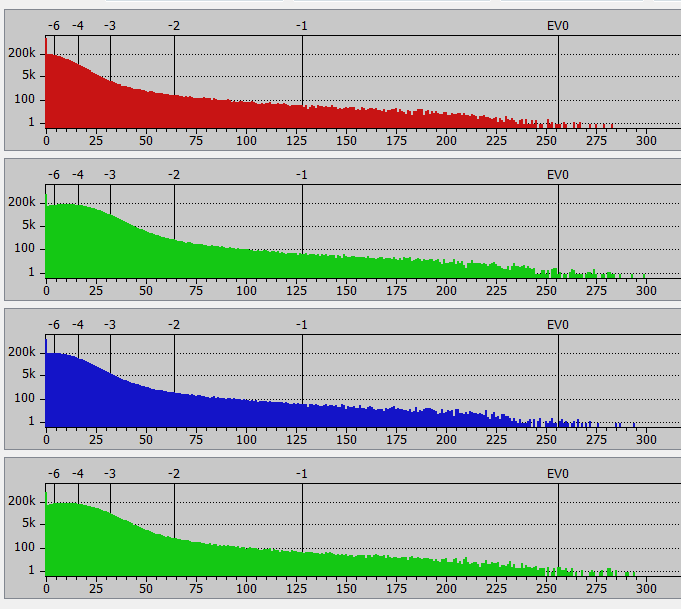
ISO 400, with a 3-stop push in ACR:

ISO 200, with a 1-stop push in ACR:

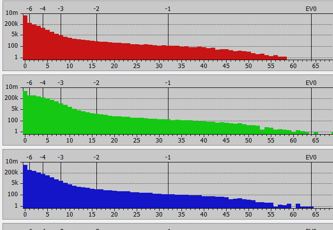
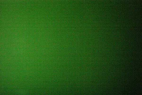
Most of the banding is horizontal, but, as the ISO goes down and the push goes up, vertical banding becomes visible. The color shift towards the green that starts with the ISO 800 image looks to be the result of truncation of the left side of the histogram. The reason that the truncation causes the green shift is that the green channels have the highest counts, so that chopping off the left side of the histogram leaves more green than blue, and more blue than red. There may be an offset, too, but I can’t verify that from these histograms.

This explains the green shadows in the pushed images of the bookcase here.

I’m sure that it’s related to the strange noise floor behavior here.