Automatic measurement of photon and read noise

I’m going to set PRNU aside, and get on with the photon transfer main event: photon noise and read noise. The reason for moving on so quickly from PRNU is not because I’ve exhausted the analytical possibilities — I’ve just scraped the surface. But with modern cameras, PRNU is not normally something that materially affects image quality. I could spend a lot of time developing measures, test procedures, and calibration techniques for PRNU, and in the end it wouldn’t make a dime’s worth of difference to real photographs. I will probably return to PRNU, since it’s an academically interesting subject, but for now I want to get to the things that most affect the way your pictures turn out.

When testing for PRNU, I took great pains to average out the noise that changes from exposure to exposure. When looking at read and photon noise, I’m going to do the opposite::try to reject all errors that are the same in each frame. That means that there is a class of noise, pattern read noise, that I won’t consider. I looked at that a month or so ago in this blog, and in the fullness of time I may incorporate some of the methods I developed then into a standard test suite.

How to avoid pattern errors.

There are two ways.

The first is to make what’s called a flat-field correcting image. The averaged PRNU image that I made in yesterday’s post is one such image. With that in hand, the fixed pattern multiplicative nonuniformities thus captured can be calibrated out of all subsequent images. This technique would not remove the fixed additive errors of pattern read noise, so it is initially appealing.

In fact, it’s the first thing I tried. After a while, I gave up on it. The problem is that the test target orientation, distance, framing, and lighting all have to be precisely duplicated for best results, and that turns out to be a huge hurdle for testing without a dedicated setup.

Jack Hogan suggested that we use an alternate technique, which works much better. Instead of making one photograph under each test condition, we’re making two, then cropping to the region of interest. Adding the two images together, computing the mean and dividing by two gives us the mean, or mu, of the image. Subtracting the two images, computing the standard deviation, and dividing by the square root of two, or 1.414, gives us the standard deviation, or sigma, of the image. Any information which is the same from one frame to another is thus excluded from the standard deviation calculation, provided the exposure is the same for the two images. With today’s electronically-managed shutters, it’s usually pretty close.

So here’s the test regime.

• Install the ExpoDisc on the camera, put the camera on a tripod aimed at the light source, and find an exposure that, at base ISO, is close to full scale. It doesn’t have to be precise, but it shouldn’t clip anywhere.
• Set the shutter at 1/30 second, to stay away from shutter speeds where the integration of dark current is significant, and not-coincidentally, where the camera manufacturer is likely to employ special raw processing to mitigate this.
• Set the f-stop to f/8 to stay away from the apertures where vignetting is significant.
• Make a series of pairs of exposures with the shutter speed increasing in 1/3 stop steps. Don’t worry if you make an extra exposure. If you are unsure where in the series you are, just backtrack to an exposure you know you made and start from there. The software will match up the pairs and throw out unneeded exposures.
• When you get to the highest shutter speed, start stopping the lens down in 1/3 stop steps until it’s at its minimum f-stop. That should give you about 9 stops of dynamic range.
• Set the ISO knob to 1/3 stop faster.
• Make another series of exposures, this time starting with a shutter speed 1/3 of a stop faster than the previous series. Do that until you get to the highest ISO setting of interest.
• Now take the ExpoDisc off the lens, screw on a 9-stop neutral density filter, and repeat the whole thing, except this time, start all the series of exposures at 1/30 second.
• Put all the raw files in a directory on your hard disk. Make sure there’s plenty of space for temporary TIFF files, since the analysis software makes a full frame TIFF for every exposure. (I may add an option to erase these TIFFs as soon as they’re no longer needed.)

That will give you a series of a couple of thousand images comprising more than a thousand pairs spanning an 18-stop dynamic range, which should be enough to take the measure of any consumer camera.

There’s a routine in the analysis software that finds the pairs, crops them as specified, separates the four (the program assumes a Bayer CFA) raw planes, does the image addition and subtraction, computes the means, standard deviation, and some derived measures like signal-to-noise ratio (SNR), and writes everything to disk as a big Excel (well, to be perfectly accurate, CSV) file.

There are several programs to analyze the Excel file, and probably more to come. I’ll talk about the most basic in this post.

What it does is perhaps best explained with an example:

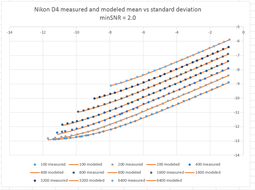
The top (horizontal) axis is the mean value of the image in stops from full scale. There are seven curves, one for each of a collection of camera-set ISO’s with whole-stop spacing (the spreadsheet has the ISO’s with 1/3 stop spacing, but displaying them all makes the graph too cluttered). The right-hand (vertical) axis is the standard deviation of the test samples, expresses as stops from one. Thus, the lower the curve, the better. The bottom curve is for ISO 100, and the top one for ISO 6400.

For each ISO, the program calculates the full-well capacity (FWC), and the read noise as if it all occurred before the amplifier – thus the units are electrons. The blue dots are the measured data. The orange lines are the results of feeding the sample means into a camera simulator and measuring the standard deviation of the simulated exposures. To the degree that the orange curves and the blue dots form the same lines, the simulation is accurate for this camera with this data.

What to leave in, what to leave out… (Bob Seger)

You will note the “minSNR = 2.0” in the graph title above. That simple expression takes a lot of explanation.

Many cameras, including the Nikon D4 tested above, subtract the black point in the camera before writing the raw file, chopping off the half of the dark-field read noise that is negative. Even ones that don’t do that, like the Nikon D810, at some ISOs, remove some of the left side of the histogram of the dark-field read noise. This kind of in-camera processing makes dark-field image measurement at best an imprecise, and at worst a misleading tool for estimating read noise.

In a camera that sometimes clips dark-field noise, with the 18 stop-dynamic-range test image set is guaranteed to have some images dark enough to create clipping. Before modeling the camera, we should remove those images’ data from the data set. It’s pretty easy for a human to look at a histogram and determine when clipping occurs, but it’s not that easy – at least for someone with my programming skills – to write code that mimics that sorting.

I tried several measures to use to decide what data to keep and what to toss, and I settled on signal-to-noise ratio (SNR). I made a series of test runs with simulated cameras that clipped in different places, and settled on an SNR of 2.0 as a good threshold. I’ll report on those tests in the future, but they are complicated enough to need a post of their own.

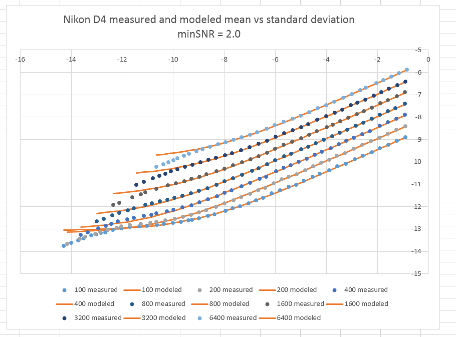
What would the curve above look like if we plotted the actual measurements that are not used to fit the model? I’m glad you asked:

You can see that the rejected blue dots on the left side of the graph are under the modeled values. This is because the rejected measurements are optimistic, since they chop off part of the read noise.

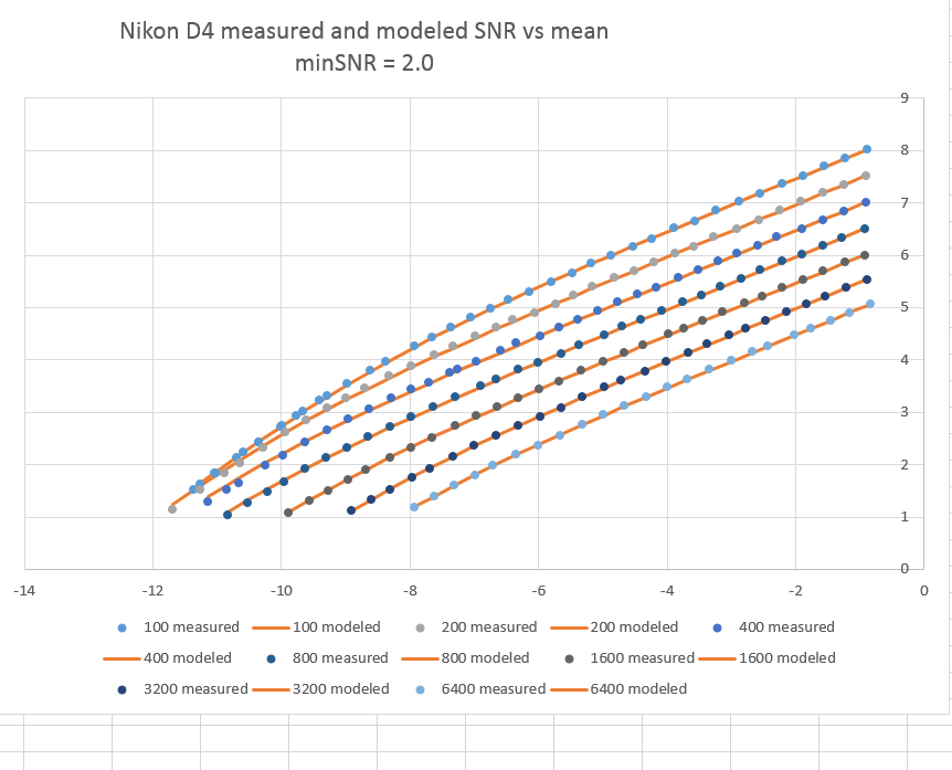
If you’re more comfortable with SNR than standard deviation as the vertical axis, here’s the data above SNR = 2 plotted that way:

Now the top curve is for ISO 100 and the bottom one for ISO 6400.

Now let’s turn to the parameters of the model.

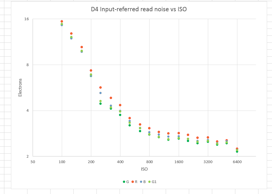
Read noise:

Except for the drop from ISO 5000 to ISO 6400, and the less significant one from ISO 200 to ISO 320, these look as expected.

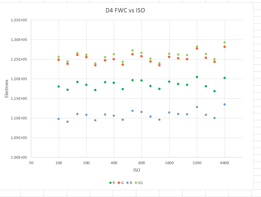
Full well capacity:

The surprise here is that the red and blue channels show slightly lower FWCs than do the two green channels. I’m suspicious that this is due to Nikon’s white-balance digital prescaling, but I haven’t tracked it down yet. It also occurs with the D810.