Camera vs sensor resolution

There’s been a lot of discussion on the web about the relationship of lens and sensor resolution. Questions often go something like, “Is putting lens A on camera B as waste of money, since lens A can resolve X while camera B can only resolve Y?” I looked around and found that there’s a body of engineering knowledge on the subject. Since it comes from the scientific imaging world, it’s aimed at equipment and usage scenarios that are different than normal photography, but it’s worth looking at.

The first assumption that’s different from most of our cameras is that the sensor is monochromatic. Thus there’s no Color Filter Array (CFA). This certainly makes the analysis easier, but we’ll need to make some adjustments to make it apply to Bayer-patterned sensors. In the applications where this approach originates, either monochromatic imaging is suitable for the task, or a filter wheel can be used to obtain color information.

The next assumption is that the lenses are diffraction-limited in their resolving power. In some scientific and industrial applications, that’s a pretty good assumption. However, many lenses commonly used in photography are not diffraction limited at wider apertures.

The last assumption is that there’s no anti-aliasing (AA) filter on the sensor. While not common in normal digital cameras, there are an increasing number that meet this test, among them the Leica M9, and M240, Nikon D800E, the Sony a7R, and all medium-format cameras and backs.

The tradeoff between camera and sensor resolution is a quantity represented by the letter Q. I will lunch room some of the concepts involved in creating and using this metric.

The first concept we need to understand is spatial resolution. The definition of spatial resolution is so small separation between two image objects that allows them to still be resolved as distinct. We need to tighten up on that definition in order to use it to quantify resolution, and the first version of that was developed in 1879 by Lord Rayleigh. The Rayleigh criterion occurs when the location of one point lies on the first zero of the Airy disk http://en.wikipedia.org/wiki/Airy_disk from the other point.

Here’s plot of a cross-section of the Airy disk plotted against x, where x = k*a*sin(theta), k = 2*pi/wavelength, a is the radius of the lens aperture, and theta is the angle from the lens axis to the point in the image plane where the intensity is desired.

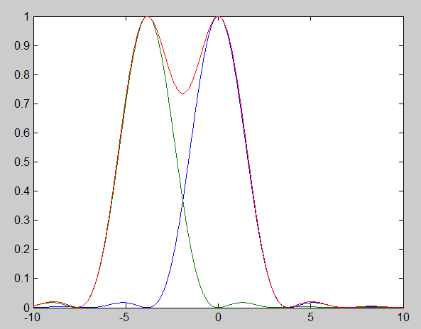
The first zero is at x = 3.83. If we plot two Airy functions that far apart – at the Rayleigh criterion, and add them together to get the red curve, here’s the intensity vs x:

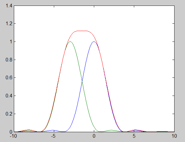
There is also another, less rigorous (in terms of separation required) spatial resolution criterion called the Sparrow criterion, which is the separation of the Airy disks where the value at the midpoint between the two disk centers just begins to dip as the disks are moved apart. That occurs at x = 2.97, and the summed Airy disks (the red curve) look like this in cross-section:

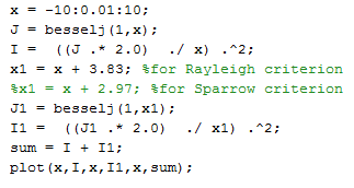
For anybody who wants to look behind the curtain, here’s the Matlab code to generate the above plots:

For photographers, x, as defined above, is not a particularly satisfying quantity. We don’t normally think in turns of angles from the lens axis unless we’re worried about coverage. We think about f-stops, not the radius of the aperture. We normally don’t think about the wavelength of light at all. Is there a way to cast the Airy disk dimensions and the two separation criteria into something that makes sense to us?

There is indeed.

After some mathematical manipulation, the Rayleigh criterion is:

R = 1.22 * lambda * N, where lambda is the wavelength of the light, and N is the f-stop.

So, for green light at 550 nanometers and the lens set at f/8 – a point where a really good photographic lens is likely to be diffraction-limited – R is 5.4 micrometers, or about the pixel pitch of modern sensors. What if we’re more stringent? For blue light at 380 nm, and the lens set to f/5.6, R is 2.6 micrometers, which is finer than the pixel pitch of current full-frame and larger sensors, though not tighter than the pitch of some smaller sensors.

The Sparrow criterion boils down to:

S = 0.947 * lambda * N, where lambda is the wavelength of the light, and N is the f-stop.

Optical engineers usually cavalierly round the 0.947 to one, giving

S = lambda * N

The Sparrow criterion is tougher than the Raleigh criterion. For our f/8 lens in green light, S is 4.4 micrometers, and for the f/5.6 lens in blue light, S is 2.1 micrometers.

So we’re done, right? Lenses with Sparrow criteria tighter than our sensors will be limited by the sensor, and lenses with Sparrow criteria looser than the sensor will be limited by the lens? That’s sort of right, if you take account of Dr. Nyquist’s teaching that you need two samples of a cycle of some spatial frequency in order to reconstruct the original.

More soon.