The a7RIV has 16-shot pixel shift technology. Fuji has said that they will be bringing that capability to the GFX 100 in a future firmware update. These events have rekindled the fires of discussion of that fifteen-or twenty-year-old scheme, specifically about how much the resolution of the system is increased. I am about to wax Clintonesque on the subject: it all depends on what the meaning of resolution is.
When I made a similar statement on a DPR board, I got a response that outwardly seemed reasonable, but didn’t survive close examination:
I’ll point you toward the dictionary for my definition of resolution.
Let’s give that a try:

Of the options, it seems only the fifth is relevant. But it has two apparently conflicting parts. The first one, that talks about the smallest interval, seems to refer to the object field. The second seems to refer to the image field. And it’s vague. It is also completely non quantitative. Could we use that definition to unequivocally say that one camera/lens systems has more resolution than another? No. Could we use it to measure the resolution of such a system? Again, no.
One measure of resolution in digital photography is simply the number of pixels per picture height or picture diagonal. It has the virtue of being simple to calculate, but in isolation doesn’t say anything precise about the amount of detail present in an image from a given camera. As an aside, the number of pixels in the sensor is not — at least in my book — a measure of resolution, but of something related.
The modulation transfer function of a system has the potential of being a precise, relevant measure of the system’s ability to record detail, but it is not a scalar.
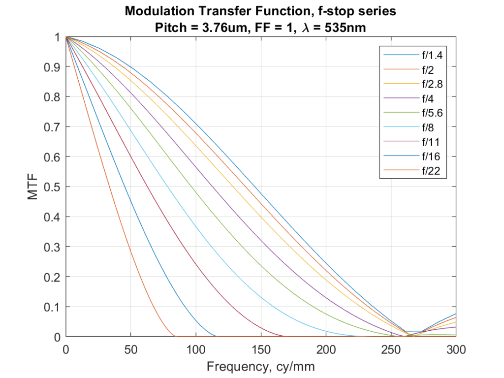
Let’s look at the MTF curves for ideal (perfectly diffraction-limited) lenses on a monochromatic sensor with a 3.76 micrometer pixel pitch and a fill factor of 100%.
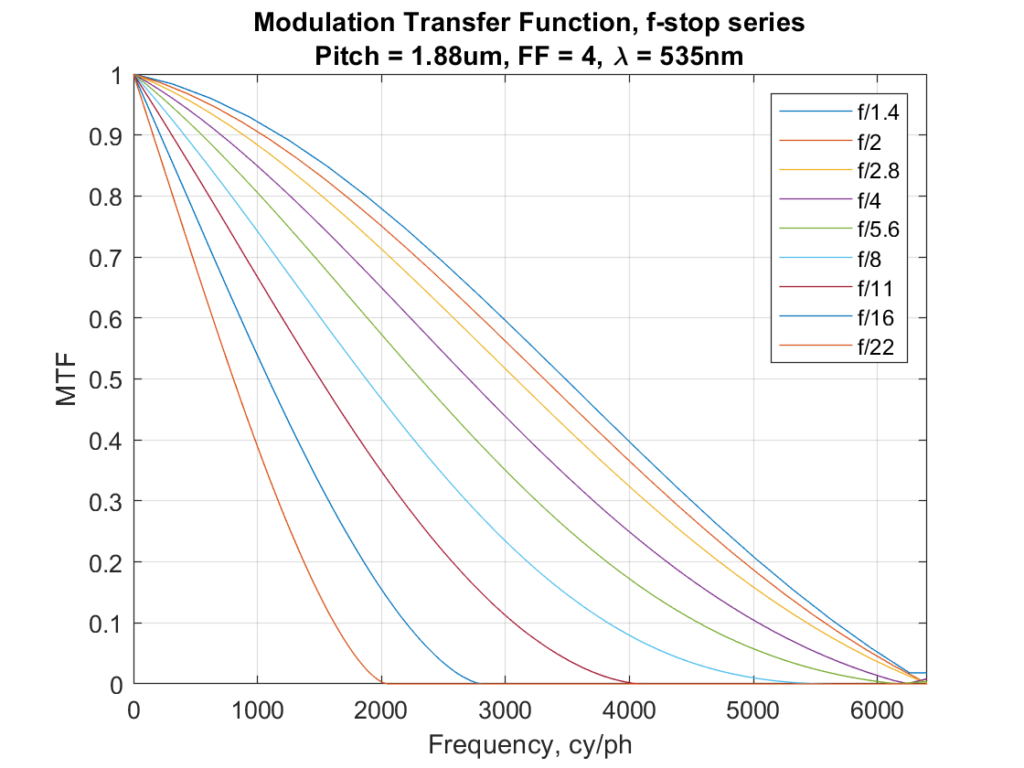
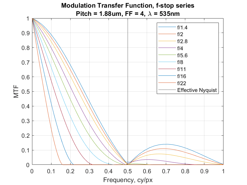
Now let’s look at the MTF of a 16-shot pixel shift image using the same sensor. This amounts to the MTF of a monochromatic sensor with a 1.88 um pixel pitch and a 400% fill factor.

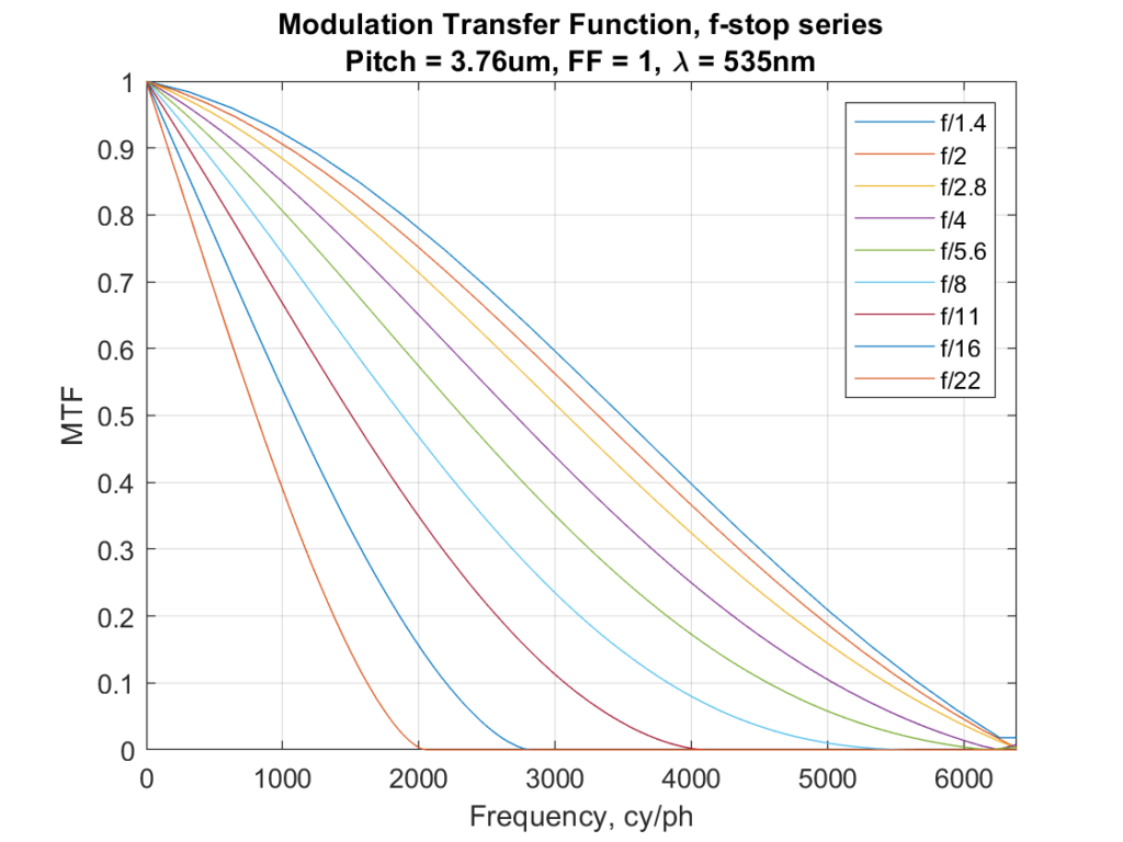
Those look very similar. In fact, they are virtually identical, and with infinite precision, they would be exactly identical. So if we’re looking at MTF in cycles per millimeter as our definition of resolution, 16-shot pixel shift buys us no resolution at all. Plotting the above image in cycle per picture height at the same scale looks similar, since the sensor doesn’t change physical size because of pixel shifting:
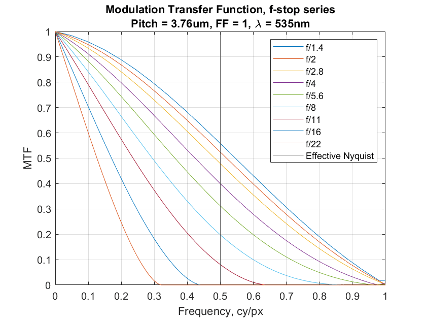
But there are important differences between the single shot and the 16-shot images. Let’s look at the MTF curves in cycles per pixel. First, a single shot.
And now a 16-shot composite:
There is a good deal more aliasing in the single-shot image.
With a Bayer-CFA sensor, there are additional advantages to pixel-shift shooting, but they are hard to quantify simply.
- The reduced aliasing in 16-shot images will allow more sharpening to be used before aliasing artifacts become objectionable.
- If the demosaicing algorithm used for the single-shot image softens edges, that will not be a problem with the 16-shot image.
- False-color artifacts will be much less of an issue in 16-shot (or even 4-shot) pixel shift images.
For more on pixel shifting, as well as real camera examples, see here.
Jack Hogan says
Good show Jim. Next I assume, in your inimitable style, will come real world samples that confirm the theoretical points? 😉
JimK says
I would do that, but pixel-shifting monochrome cameras seem to be a little thin on the ground.
FredD says
@Jack Hogan:
With regard to “real world samples that confirm the theoretical points”, IIRC, it was you a few years ago who posted on a DPR forum a comparison of different treatments of the “aliasing hell” engraving portion of the DPR studio test shot. IIRC, you compared, for the Pentax K-1, a single shot with linearization-equalization of the three color channels in post vs. a pixel-shifted shot. Obviously, that only works with a B&W subject (and though etch-line aliasing is not the same as grain-aliasing, still might be of some relevance for the digitization of B&W negatives). Any chance that you (or Jim) could, using your same methodology, do a similar comparison for the A7R4? (And to make it even more interesting, compare that to your old K-1 results? (to see what all those extra megapixels and double the price bring!)).
Erik Kaffehr says
Thanks for the demo!
So, my take is that doing the 16x multishot essentially doubles the sampling frequency and the pixel aperture essentially functions as a low pass filter.
My perception, right now, is that the perceived increase in resolution may be the reduction of artifacts, combined with possibly better demosaicing.
Best regards
Erik
JimK says
And more opportunity for sharpening without creating ugliness.
Ilya Zakharevich says
A lot of thanks for putting nice illustrations to what I said on DPR!
One moment is puzzling me, though: given that you confirm EVERY point I said, how come you write:
“outwardly seemed reasonable, but didn’t survive close examination”
?
JimK says
Ilya, are you also Rick?
Ilya Zakharevich says
Oups, do you mean your were answering somebody else?! Sorry then…
Trying to find this thread again… (The search on DPR is not very helpful at all…) Nope, no Rick contributed there. So: why do you ask?
And: I’m always ilyaz — unless some impostor already took this.
JimK says
Then I wasn’t talking about you.
Ilya Zakharevich says
LOL! You are absolutely right! What I actually wrote is:
“The reason for double-think is the meanings of the words.”
— which is a bit different from what Rick wrote in
[edited out, sorry Ilya]
Sorry for a confusion!
Hans van Driest says
Say you have a sensor with 3 pixels, all with the same size and in a line. On the sensor is projected a narrow (compared to the pixel size) line, at right angles to the line of pixels. The pixels are numbered 1, 2 and 3. The position of the line is 1/4th after the start (side) of pixel 2.
Now let’s introduce pixel shift of half a pixel, in the direction of the line of pixels. We get pixel 1/1a/2/2a/3/3a. The same line is still there. The line will be visible in pixel 1a and 2. The (closest) surrounding pixels where the line is not visible are pixel 1 and pixel 2a, and we know the distance between these two is only half a pixel. From this we can know the position of the line to within half a pixel. Maybe I am missing something, but to me this seems like more resolution. A drawing would have been better, but do not know how to add this to a comment on your site.
JimK says
The only works if you have a priori knowledge of the nature of your subject (the line). And it amounts to sharpening in post.
Ilya Zakharevich says
Sorry, but I cannot agree with this. You cannot watch RAW files. You need postprocessing. And if a part of the physical pipeline is blurring, the part of the postprocessing pipeline should be sharpening.
AND: you cannot deRAW without “a priori knowledge of the nature of your subject”. Moreover, AFAICS, the STANDARD assumptions used in deBayering would make the argument above work.
JimK says
You can process raw files for MTF one raw plane at a time. That’s the way I often do it for lens testing. No post processing required, except x = y(1:2:end,1:2:end).
Hans van Driest says
Sorry, pushed the post button too fast. What I mean is that it seems to me that by the propper math on the result, a higher resolution seems obtainable.
In some results I have seen on the internet, from Sony A7r4, the resolution with pixel shift seems to really be increased (for example result by Tony Northrup).
kind regards,
Hans van Driest says
Hi Jim,
I have been thinking a bit more on this, and been drawing more diagrams. If I take the same 3 pixel line sensor, and project 3 lines on it (double the spatial Nyquist frequency), shifting the sensor half a pixel size does not resolve anything more, so that is where you are obviously right, the resolution does not increase, not in the sense that a higher frequency can be observed as such.
But now the same 3 pixel line sensor, and an edge (a transition from white to black or the other way around) over it, say a transition at 3/4th of the second pixel. Without pixel shift this edge covers both pixel 2 and 3, we can not know more about it. With half a pixel shift, the edge will also cover pixel 2 and 3. But now we do no more. If the transition would have occurred at 1/4the of the second pixel, it would make no difference without pixel shift, but with half a pixel shift (to the right, in my diagram), the edge will now only occur in pixel 3. So, we do not know more about the frequency (due to the hold filter as a result of the pixel size), but we do know more about the position of the edge. This could explain why an image with pixel shift, in examples I have seen, look more detailed. With a 2 dimensional sensor with pixel shift a circle or slanted edge will be resolved better/more accurate.
Kind regards,
JimK says
The reduction in aliasing provided by the pixel shifting does indeed allow you to know more about the scene, if there is information about the Nyquist frequency of the unshifted sensor. Try to come up with an example where there is no information above that frequency.
Hans van Driest says
For ease of communication it would perhaps be better to think of the pixel shift on a line sensor, as if it were an electrical system with two AD converters with each a S/H, where the hold equals the sample interval (giving you the equivalence of a pixel with 100% fill factor), and the second S/H samples, half a sample interval shifted
If the input are pulses with a frequency of 1.5 times the Nyquist limit and we take four samples with only one ADC, and the first pulse occurs at 3/4th of the first sample, the output would be 1010.
If we would sample the same signal with the two converters (of which one is one sample period shifted), we would get 11011011. So here it is clear the magnitude of the output is reduced.
This example illustrates the reduced aliasing, I think.
If we stay with this analogy, you are looking in the frequency domain, and I look in the time domain.
When in the above example I apply a transient, say in sample 2 (of the single sampler) at 3/4th of the second sample, the output will be 0100. When I now add the signal of the second sampler, and again represent its output as an extra bit, in between the bits of the first sampler, I get 00111111. When I now shift this transient half a sample (to 1/4th of the second bit), I get 0111 in the single output (the same) and 01111111 with the two samplers. So there really is more information on where the transient takes place. I do not know of a way to achieving the same result with an anti-aliasing filter, simply because the time domain information is not there.
I think pixel shift not only reduce aliasing, it also adds information.
Kind regards,
JimK says
A sample and hold circuit is a time-domain analog to a spatial point sampler. To come up with a time-domain analog to a spatial sampler with a fill factor of 100%, you’d have to average the previous time period’s signal, not just sample it. But the key issue with you example is that it contains frequencies in excess of the Nyquist frequency. Come up with another example that stays under the Nyquist frequency for the unshifted sensor, and I think you’ll see that the shifting doesn’t improve the MTF.
Hans van Driest says
Have made a simple model with Excel, and found the same result as shown in the first part of this article.
https://www.vision-systems.com/cameras-accessories/article/16735762/pixel-shifting-increases-microscopy-resolution
I think it should be possible to reduce the sidelobes, but even as is, it does increase positional accuracy. Maybe not so much increase resolution itself, although it very much looks like it does, in a detailed photograph. Looking at the results as shown by DPR, in for example the review of the A7R4, I find the pixel shift result look ‘better’, even compared to the 100Mp Fuji.
Anyway, I do not own a camera capable of pixel shift, and it seems cumbersome in use.
Ilya Zakharevich says
First, YOU need to come up “with an example where there is no information above that frequency”. This would mean something strongly diffraction-limited (about ƒ/8 with current sensors). Possible — but WHY discuss such a case?
JimK says
I don’t mean find a lens and setting that will eliminate aliasing for all subjects. But you’re trying to prove that pixel shift helps even setting aside its ability to reduce aliasing. So you’ll have to produce an example where there is no aliasing.
Hans van Driest says
Hi Jim,
Was planning to let go of this pixel shit thing, but came up with another idea anyway. Idea about how to combine the four shifted images.
I made a simple model in Excel. The input resolution is double the pixel size, so it takes four positions (2×2) in the 2D input matrix, to cover a full pixel. The output is the average of four pixels (2×2), to behave like a normal pixel would. Shifting one input sample (half a pixel), to the side and one down and to the side, creates four versions of the single input matrix in the output, each a 1/4th the input value.
I started out by creating an output by adding up the four values of the four shifted versions, for each quarter pixel position. An input of:
0 0 0 0 0
0 0 0 0 0
0 0 4 0 0
0 0 0 0 0
0 0 0 0 0
Results in:
0 0 0 0 0
0 1 2 1 0
0 2 4 2 0
0 1 2 1 0
0 0 0 0 0
The numbers represent light intensity (for example).
The interesting thing with the above scheme, is that shifting the input by half a pixel, also shifts the output by half a pixel. Where in the case of a normal output, without pixel shift would result in:
0 0 0 0 0
0 1 1 0 0
0 1 1 0 0
0 0 0 0 0
0 0 0 0 0
Or a shifted version of this. And moving the input halve a pixel would either not move the output (because the input is still on the same pixel), or shift a whole pixel position (double the move of the input).
This worked, but I do not like the way the pixel is expanded.
I came up with another way to interpreted the input; look only on what the four shifted versions share, at a single position, or the lowest value of the four. Not very good for noise, and non-linear, but it gives nice results:
0 0 0 0 0
0 0 0 0 0
0 0 1 0 0
0 0 0 0 0
0 0 0 0 0
When the input is shifted half a pixel, the output shifts by the same amount. The value is however reduced to a quarter of the input, and only when the input is covering more area, the output will clime to the 4 of the input. What is also interesting, is the following input:
0 0 0 0 0 0
0 0 0 0 0 0
0 4 0 0 4 0
0 0 0 0 0 0
0 0 0 0 0 0
This will result in:
0 0 0 0 0 0
0 0 0 0 0 0
0 1 0 0 1 0
0 0 0 0 0 0
0 0 0 0 0 0
Shifting both values half a pixel in any direction will result in the same shift in the output. Both input and output are above the Nyquist limit, related to the pixel size. This seems remarkable.
Will not give more examples, this replay window is a bit impractical for this.
Hans van Driest says
link to Excel sheet with model.
left top is input, below that is output without pixel shift, bottom right is result with pixel shift.
https://ufile.io/xrcff5yi
kind regards
Hans van Driest says
Hi Jim,
I must admit to find it a bit frustrating you don not reply anymore. I should probably have put in more effort before my first reply, but by now I have put both effort and thought in this. Thought in how to combine the four shifted results. And I think my latest result/example (in the spread sheet), clearly shows how pixel shift does not give the same result as say double the number of pixels, but a much-improved result compared to unshifted. And the later not only in reducing artefacts/aliasing
Have re-read your latest comment, to see if I missed something. I am not completely sure I do understand you, but keeping the spatial frequency, at the input, below the Nyquist boundary for the unshifted sensor could hardly give an improvement in resolution, since there is no possible improvement with a higher resolution sensor, apart from reducing artifacts/aliasing.
Kind regards
JimK says
I never said that pixel shift didn’t create better images. I merely said that, before sharpening, the improvement is not due to increased resolution, but decreased aliasing.
The reason I stopped replying is that you never took my advice to separate aliasing and resolution, and produced examples that conflated the two.
Your statement that, keeping the input below Nyquist, the sensor doesn’t matter (generalizing whatt you said) is untrue, if the definition of resolution is, as in the original post, the MTF curve below Nyquist. Pixel aperture, for example, has a strong effect on the MTF curve below Nyquist.
Hans van Driest says
Hi Jim,
I reread your article, worried I missed something (and I am sure I did miss things). The thing a noticed for the first time, is something in the MTF curves I did not expect. You show an MTF for a sensor with a 3.76um pixel pitch, and below that an MTF for a sensor with half the pixel pitch, and a fill factor of 4 (I assume four times the area, double the linear size). These curves are identical. And for me this is confusing.
In the more traditional use of MTF, say for a film, the input and output frequency are the same. So, the spatial frequency as visible on the film after development, is the same as the one projected on it during exposure. In a digital system this is more complicated. There is the pixel dimension, a rectangular filter, which gives a sinc(x) frequency transfer (the transfer that is an upper limit in your plots, when no lens would be present). But a digital sensor is also a sampled system with an upper limit to the frequency transfer, often called the Nyquist limit, or such. I can only assume that in your plots, the x-axis shows the equivalent of input frequency, and the y-axis shows the amplitude at the output of the sensor. Where your plots to show the output frequencies, they would be totally different, in that the first plot would simply stop, halfway the x-axis, since there is no signal above that frequency. The input signal with a spatial frequency above the halfway point, would be folded back (aliased) to a lower frequency.
I am sure the way you show it, is the way MTF is used for digital systems, but used this way it does not tell you much about the resolution of a system. Resolution in the sense of highest spatial frequency that can be reproduced, something like lines/mm, at the output of the system.
What I tried to show in my previous examples, is how pixel shift does resolve detail above the Nyquist limit of a non-shifted system.
Kind regards,
JimK says
Consider that the MTF is the absolute value of the Fourier transform of the point spread function. The equivalent of the post spread function of the sensor/lens system is the convolution of the point spread function of the lens with the effective pixel aperture of the sensor. Notice that the pitch of the sensor doesn’t figure into any of that. So it makes sense that sampling more often with the same pixel aperture won’t change the MTF.
I am not saying that it doesn’t.
Hans van Driest says
‘Consider that the MTF is the absolute value of the Fourier transform of the point spread function. The equivalent of the post spread function of the sensor/lens system is the convolution of the point spread function of the lens with the effective pixel aperture of the sensor. Notice that the pitch of the sensor doesn’t figure into any of that. So it makes sense that sampling more often with the same pixel aperture won’t change the MTF.’
What you describe is the MTF for the linear part of the system, it completely ignores the influence of sampling part to the frequency transfer.
The pixel aperture gives a first zero (in the spatial frequency response) at 1/(pixel aperture), and the bandwidth will be infinite. At the output of a sampled system, the highest frequency to be reconstructed is 1/(2*sample aperture).
In other words, the MTF for the linear part of the system, does not tell much about the resolution of the total system.
JimK says
in the general case, that’s not true at all. If we’re talking meaningful results, the highest frequency to be reconstructed is half the sampling frequency, and is unrelated to the aperture. Consider, for example, a point sampler.
Mike Joyner says
Thanks Jim for a firm grasp on actual (real) resolution. With the current system bottle neck at the spot size performance of the lens, the megapixels wars has been and continues to be marketing nonsense.
The pixel shifting mode to me as a sensor designer is novel in reducing aliasing, and color reproduction. That is beneficial for perceived resolution and improved color extraction. Color filter size is another factor as smaller is not better in filter function. Given crosswalk becomes more prevalent as pixel size is reduced against a decreased full well both optical cross talk and signal cross talk (in the column amplifiers up until A/D conversions.) I would submit the more significant benefit would be when pixel size approached the spot size of the lens in use.
JimK says
I have not found pixel shift useful in the field. Too many motion artifacts. I think the solution is to get the pitch down more. With BSI, I’m not seeing any CFA crosstalk at 3.76 um pitch. FWC per unit area is not strongly dependent on pitch.
JimK says
This is far from being the case, at least on-axis with decent lenses at reasonable apertures. With many of the lenses I have, we’re going to see significant aliasing even with 2 um pitches.
JimK says
I disagree. The files I’m getting from the GFX 100 are far superior to those from the GFX 50x, because of the reduced aliasing.
Isee says
I think this proves what I have figured out by just common sense: one cannot attain much more contrast resolution than the physical pixel can attain.
That is, moving the same size pixel around cannot provide much more “real” contrast resolution, as it does not get physically smaller to get exact readings of details smaller than itself.
E.g. Here we have 3.76um pixel. Lets assume we have a totally black detail on totally white background that is width of 2 um. Now, at best, we can sample both sides of the detail, and get value 255 (8bit), and then we can arbitrarily place the pixel on top of that detail with about the same result that will be something like 120 ((1 – 2/3.76)*256) as the detail is smaller than the pixel and hence that detail will “shadow” the pixel partly. No matter how we move the 3.76um pixel, we cannot reconstruct the detail precisely, only as “there’s likely something there, blocking some of that reflected/incoming light”
So at best we get a vague smear on our recording. In practice we would get even more smear as we likely won’t be able to achieve such precision in the sampling that we’d get samples exactly around the detail. So it would be shadowing the sampling on more samples and on “wider area” of the pixel shifting than ideally we would want to, causing more smear.
Now, I am sure some clever signal processing and huge sample count of small shifts will be able to improve the situation. So that we can figure out precisely where the detail starts to shadow and via that “draw” the detail precisely (but not necessarily in correct brightness). But when we have more of these 2um details at 2um away from each other, I believe there’s nothing one can do, as the pixel will always have at least one detail “shadowing” it, and the end result will be wavelike grey varying between something above 0 and 120.
I purposefully ignored microlens in this example. That will inevitable further smear things up.
However, we can also get the intrapixel region sampled, but the benefit for resolution of this is unclear for me.
To me, the biggest benefit of pixel shifting is to improve color accuracy by sampling full RGB over Bayer CFA.
Also in GFX100 case, it should get rid of the PDAF banding to great degree.
Jan Steinman says
Having worked in DSP (synthetic aperture sonar), I don’t think your charts are telling you what you think they are telling you.
While it is true that the pixel pitch (sampling aperture) is fixed, one can synthesize a smaller sampling aperture. It’s been a long time since I read Shannon, but I believe it involved a cosine function. (Of course, with the technology of the day — MC68000 processors — we did it with look-up tables.)
Although your charts show a different pixel pitch, I don’t understand why that would not result in increased frequency discrimination. Perhaps MTF isn’t really measuring that, or there is something else going on. You correspondingly change the “fill factor”, which may have simply nullified the pixel pitch. As I mentioned, synthetic apertures have been a “thing” since at least the MC68000 days, so I don’t understand why it would suddenly stop working on modern digital cameras!
I think the system resolution is the square root of the inverse of the sum of the squares of the individual component resolutions. This means that the system resolution can only approach the resolution of the least-resolving component.
So if you stick a lens on there that cannot resolve one half the frequency of the sampling aperture, there will be nothing gained. That’s pretty easy to verify.
It is also pretty easy to verify that if you put a lens capable of resolving significantly better than 1.88µm, you should see increased resolution with oversampling and synthetic aperture.
Perhaps I’m missing something important here. But similar DSP techniques have been used for at least 40 years to increase effective resolution.
Jan Steinman says
Perhaps reviewing how synthetic aperture radar works could be insightful.
This website shows how details of a ship can be discriminated that could not normally be discriminated, via oversampling and synthetic aperture processing. This sounds quite a bit like how high res through sensor positioning works!
Jan Steinman says
Perhaps reviewing how synthetic aperture radar works could be insightful.
This website shows how details of a ship can be discriminated that could not normally be discriminated, via oversampling and synthetic aperture processing. This sounds quite a bit like how high res sensor positioning works!