There is a widespread belief about Bayer color filter array (CFA) response spectra. It goes something like this:
- The old CCD cameras used to have great color.
- The reason they had such good color is the dye layers in the CFA were thick.
- Thick dye layers led to highly selective (narrow band) spectral responses.
- Modern CMOS cameras have lousy color.
- The reason is that they are trying to reduce photon noise in the images.
- Making the CFA filters less selective reduced the photon noise, but made the colors bad.
I have seen no evidence that the color is better — which, for the purpose of this post, I’ll define as more accurate — on old CCD cameras than it is on new CMOS ones. I’ve owned and used several old medium format CCD cameras and backs, and I don’t think the color was more accurate.
I decided to apply some analysis to the issue. Jack Hogan has demonstrated that you can get pretty darned close to a Macbeth CC24 Sensory Metamerism Index (SMI) of 100 with three Gaussian spectral responses of well-chosen peak wavelengths and standard deviations. I fired up a Matlab simulator that started a long time ago with some code I got from Jack, made some changes, and found such an optimal CFA response set for the CIE 1931 2-degree Standard Observer:
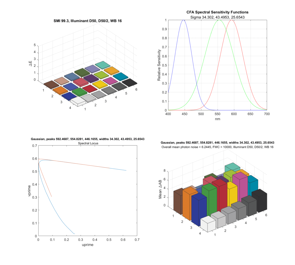
There are four quadrants in the above chart. On the top right is the response of the optimal Gaussians. The standard deviations in nanometers are given in the subtitle. To the left of that is the error, in CIELab DeltaE 2000, for each of the Macbeth CC24 patches, with an optimal compromise matrix. The overall SMI, 99.3, is shown. A perfect SMI is 100. I’ve never seen a real consumer camera get above the low 90s. Most real cameras are in the 80s. Below that, on the left, in red, is the response of the simulated camera and compromise matrix to a range of spectral inputs spanning the visible wavelengths. The blue curve is the correct response.
The bottom right graph needs some explication. I simulated a camera with a full well capacity of 10,000 electrons, or a camera with a FWC of 40,000 electrons at two stops above base ISO. I simulated an exposure sufficient to illuminate the raw values of the lightest gray patch to 95% of full scale. I simulated a 40,000-pixel patch, and, assuming a Poisson distribution for photon counting, measured the mean chroma noise in CIElab DeltaAB. The average for all 24 patches is a bit over 6 DeltaAB.
Now let’s tighten up the standard deviations, and make them all 20 nm. Then we’ll search for the optimal wavelengths for the peaks:
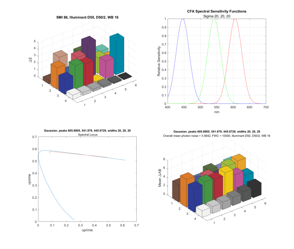
The color accuracy is much worse, but about the same as many consumer cameras, and the noise is slightly better. This is with the same exposure as the top chart. Since the filters are more selective and less light is hitting the sensor, the signal to noise ratio of the photon noise is worse, but the compromise matrix means that that degradation doesn’t result in greater chroma noise.
If we tighten the standard deviations down to 10 nm and reoptimize the peak locations, here’s what happens:
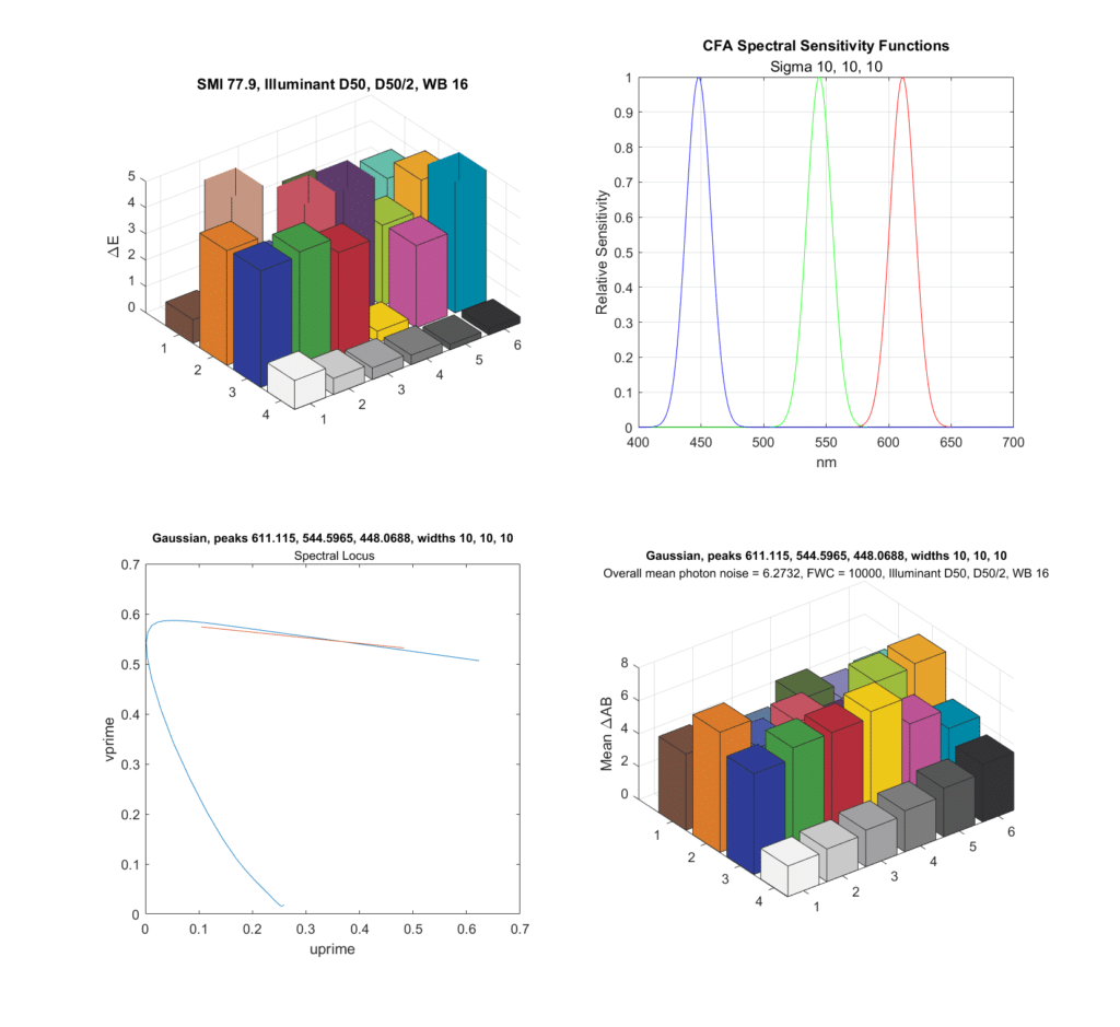
Now both the SMI and the chroma noise is worse, and the locus of spectral colors is very short.
What happens if we make the standard deviations large?
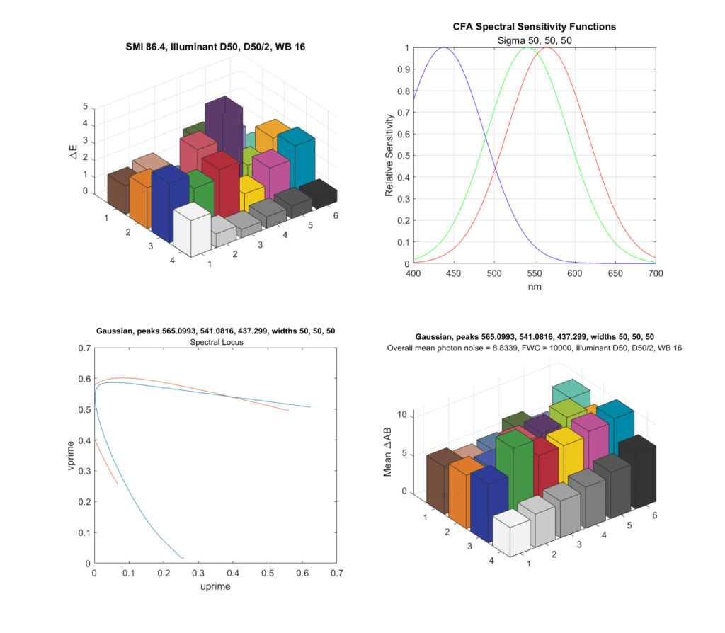
The SMI isn’t too bad, but the chroma noise is worse, in spite of more light hitting the sensor. The spectral coverage looks pretty good.
Here’s the reason for the increased chroma noise:
Note the size of the off-diagonal terms.
Here are my conclusions from this exercise:
- Too much overlap is bad for color accuracy.
- Too little overlap is bad for color accuracy.
- For optimal SMI performance, the red and green center wavelengths should be fairly close.
- For optimal SMI performance, the red and green overlap should be larger than we see in most cameras.
- You can achieve remarkably high SMIs — much higher than we see with consumer cameras — with simple Gaussian spectra.
- The CFA spectra for high SMI isn’t that far off the CFA spectra for low chroma noise.
- My guess is that the reason we don’t have better SMIs in consumer cameras is the availability of chemical compounds, not noise considerations.
Caveats:
- I optimized and tested with the same patch set. This is not ideal.
- 24 patches is a small number.
- I didn’t simulate demosaicing.
N/A says
hmm… people talk about “color” after LUT profiles, not after linear matrix color transform… so granted when you have good results with plain matrix it is telling but still not the same and then nice gaussian curves still not exactly the same as real SSFs – who knows may be “wider” “real” curves are indeed worse than “thin/selective” “real” curves – vs what you show with non-real SSFs ?
JimK says
You can use LUTs to correct errors in linear transforms. I would think that CFAs that need little correction would be better than those that need a lot.
N/A says
you can, but for example this is not what ACR/LR do (for quite a long time) in their DCP profiles supplied by Adobe … their matrix transforms (pre LUT) are intentionally are not optimal (if left alone)… so in real life LUT do not correct errors they actually do the job
JimK says
None of the Adobe profiles are even attempting to create accurate color.
JimK says
Let me expand on the above. If a camera meets the Luther-Ives condition, which means that the CMF/sensor spectra are a linear transform of CIE XYZ, that means that the camera will not see colors that appear different to a color-normal observer as the same color. If the camera sees two different colors as the same color, no amount of LUT tweaking will separate them.
CarVac says
In implementing white balance in my photo editor Filmulator, I noticed one specific difference between old camera models and newer ones: new cameras have much more overlap between the green and blue color channels, so that the white balance multiplier for the blue channel can be less extreme in warm light conditions.
It is the difference between a blue channel multiplier of 4 or so for a modern sensor and perhaps upwards of 10 for an older 2005-era sensor, which can make a huge difference in perceived noise in real-world low light conditions.
Jack Hogan says
Excellent Jim, your results in the first Figure are pretty close to what I got. What minimization criteria did you use to determine the ideal gaussian means and standard deviations?
JimK says
Just the simplex method. It’s possible there are global maxima for CRI that are greater than 99/3, but the curves are pretty smooth.
Note that I used a different Standard Observer than you did.
Tucker Downs says
I’d be curious to see your results with a much larger dataset than the CC24, but great work and simple demonstration nonetheless. And would you look at that, your ideal gaussians are extremely similar to the LMS cone sensitivities. Not surprising at all. XYZ based on color matching experiments is a good practical approximation of our color sensitivities, but the true inputs to our visual system are strictly the positive-value absorption spectra of the cones. None of the red “bump” in short wavelengths that is present in the XYZ system (for good reasons).
Anyway to make a long story short, if allow for a freeform optimization that tweaks each of those sensitivity curves at 10nm intervals, using your ideal gaussians as the starting data. I’m sure your match will get even closer to the cone sensitivities.
Glad I checked back in on your blog! As a color scientist I look forward to reading the next few posts in this sequence this afternoon.
JimK says
Thanks. Stay tuned for lots more patch sets.
JimK says
You may be interested in this thread.
https://www.dpreview.com/forums/post/66037974
Tom Lewis says
Hi Jim,
I’m interested in false color imaging derived from the near infrared. I have learned that some folks have used filters from Midwest Optical and MaxMax for this purpose. They take three photos with the filters, convert each to monochrome, and then assign to BGR in an application like Photoshop. Seems to me an objective should be to have sufficient overlap and shallow enough filter skirts to provide a wide variety of resulting visible color. But since this is false color, I can’t imagine how there could be serious criteria for color accuracy.
I have noticed that most of the filter responses for real cameras designed for visible light have overlap between 40% and 80%, and are peaky (non flat passbands). While the Midwest Optical bandpass claim to be gaussian, their spacing and standard deviation don’t appear to provide for enough overlap. In the case of the MaxMax set, the overlap occurs around 10%, and two of their filters look to me to not be designed to be gaussian.
https://midopt.com/filters/bandpass/
http://www.maxmax.com/filters/bandpass-ir
Do you have any thoughts on optimum filter combinations for humans to see purely the near infrared with false color?
Tom
JimK says
Since color accuracy doesn’t apply here, then you can use any filter skirts you please. However, there should be some overlap to avoid posterization. Keep in mind that, by 850 nm, most CFA filters are transparent, so for long lambda IR, you don’t need to convert the camera.
Tom Lewis says
Thank you, Jim.
At around what percent transmission do think would be good for the overlap to minimize posterization?
When I suggested non-vertical skirts would be a benefit, I was thinking these would provide encoding for intermediate colors. In contrast, if the filters had absolutely flat pass bands and absolutely vertical skirts, then it seems to me the system would only be able to encode three discrete colors in total, and there would be no intermediate colors. I was thinking to distinguish intermediate color, encoding a value into more than one wavelength band would be necessary.
When you mentioned no need to convert the camera for long lambda IR, I’m assuming you are referring to conversion to monochrome, and not referring to conversion to full spectrum. Is that right?
JimK says
There should be material contribution from at least two bands at every wavelength.
We’re on the same page here.
Right.