• site home
  • blog home
  • galleries
  • contact
  • underwater
  • the bleeding edge

the last word

Photography meets digital computer technology. Photography wins -- most of the time.

You are here: Home / The Last Word / How Sensor Noise Scales with Exposure Time

How Sensor Noise Scales with Exposure Time

May 12, 2025 JimK Leave a Comment

When you increase the exposure time in a digital camera, you expect to collect more signal. But what happens to the noise? The answer depends on the source of the noise. Understanding how each one scales with exposure time helps you optimize your imaging strategy, especially in low-light or long-exposure situations.

Let’s look at the major noise sources in a CMOS image sensor and how they behave as exposure time increases.

Noise Source Scales with Time? Behavior
Read Noise No Constant per frame
Photon (Shot) Noise Yes Increases as √(signal)
Dark Current Shot Noise Yes Increases as √(dark current × time)
PRNU (Photo Response Non-Uniformity) Mostly no Fixed per signal level
Thermal Drift / Bias Instability Maybe Depends on system design

In more detail:

Read Noise: Constant Per Frame

Read noise is generated during the readout process, not during integration. It’s a fixed cost for every exposure, whether it’s 1 ms or 10 seconds.

Longer exposures make read noise less significant because it’s swamped by other time-dependent noise.

Photon (Shot) Noise: √Signal

Photon noise comes from the random arrival of photons. It increases as the square root of the number of photons detected, which itself increases linearly with exposure time (assuming constant illumination):

σ_photon ∝ √(exposure time)

This means that SNR improves with √time — doubling exposure improves SNR by about 1.41×, not 2×.

Dark Current and Its Noise: Linear + √Time

Dark current is a signal-like contaminant — it builds linearly with time and adds shot noise just like a real signal. The noise it introduces behaves like:

σ_dark ∝ √(dark current × exposure time)

Longer exposures result in:

  • More dark current signal,
  • More dark current shot noise,
  • Greater risk of hot pixels and fixed pattern artifacts.

Cooling the sensor reduces this component dramatically, as shown in the previous post.

PRNU: Independent of Time

PRNU scales with signal, not time directly. So, while a longer exposure increases the signal and therefore the PRNU noise (σ_PRNU ∝ signal), the relationship is indirect. PRNU doesn’t depend on integration time per se, but only on how much signal is accumulated.

In some sensors, very long exposures can introduce bias drift or low-frequency noise (e.g., 1/f effects or leakage from imperfect bias circuits). These effects are:

  • Often sensor- or system-dependent,
  • Exacerbated by thermal instability,
  • Difficult to model precisely.

In most modern sensors, these are negligible under typical conditions but may become visible in minutes-long exposures.

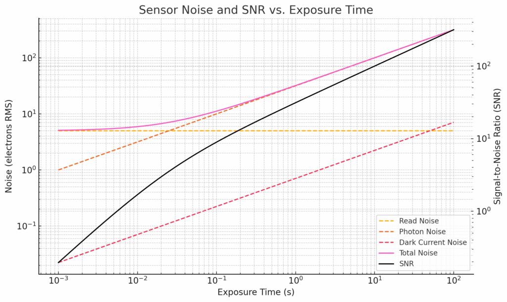
Let’s say you start increasing exposure time from 1 ms to 1 second to 10 seconds. Here’s what you can expect:

  • Signal: Increases linearly with time.
  • Photon noise: Increases as √time.
  • Dark noise: Also increases as √time.
  • Read noise: Stays fixed — becomes less important over time.
  • SNR: Improves with √time — but slowly.

Practical Implications

  • At short exposures, read noise dominates. That’s where high-conversion-gain (HCG) modes shine.
  • At medium exposures, photon noise dominates, and you’re approaching the ideal shot-noise limit.
  • At long exposures, dark current and its noise start to intrude — unless you cool the sensor.
  • PRNU and fixed pattern become visible at high signal levels, regardless of time.

Increasing exposure time is a powerful tool for improving signal-to-noise ratio, but it interacts differently with each type of sensor noise. To get the most from your camera, you need to understand not just what noise is present — but how it evolves over time.

The Last Word

← Dark Current in CMOS Sensors: Where It Comes From, and How Cooling Helps

Leave a Reply Cancel reply

Your email address will not be published. Required fields are marked *

May 2025
S M T W T F S
 123
45678910
11121314151617
18192021222324
25262728293031
« Apr    

Articles

  • About
    • Patents and papers about color
    • Who am I?
  • How to…
    • Backing up photographic images
    • How to change email providers
    • How to shoot slanted edge images for me
  • Lens screening testing
    • Equipment and Software
    • Examples
      • Bad and OK 200-600 at 600
      • Excellent 180-400 zoom
      • Fair 14-30mm zoom
      • Good 100-200 mm MF zoom
      • Good 100-400 zoom
      • Good 100mm lens on P1 P45+
      • Good 120mm MF lens
      • Good 18mm FF lens
      • Good 24-105 mm FF lens
      • Good 24-70 FF zoom
      • Good 35 mm FF lens
      • Good 35-70 MF lens
      • Good 60 mm lens on IQ3-100
      • Good 63 mm MF lens
      • Good 65 mm FF lens
      • Good 85 mm FF lens
      • Good and bad 25mm FF lenses
      • Good zoom at 24 mm
      • Marginal 18mm lens
      • Marginal 35mm FF lens
      • Mildly problematic 55 mm FF lens
      • OK 16-35mm zoom
      • OK 60mm lens on P1 P45+
      • OK Sony 600mm f/4
      • Pretty good 16-35 FF zoom
      • Pretty good 90mm FF lens
      • Problematic 400 mm FF lens
      • Tilted 20 mm f/1.8 FF lens
      • Tilted 30 mm MF lens
      • Tilted 50 mm FF lens
      • Two 15mm FF lenses
    • Found a problem – now what?
    • Goals for this test
    • Minimum target distances
      • MFT
      • APS-C
      • Full frame
      • Small medium format
    • Printable Siemens Star targets
    • Target size on sensor
      • MFT
      • APS-C
      • Full frame
      • Small medium format
    • Test instructions — postproduction
    • Test instructions — reading the images
    • Test instructions – capture
    • Theory of the test
    • What’s wrong with conventional lens screening?
  • Previsualization heresy
  • Privacy Policy
  • Recommended photographic web sites
  • Using in-camera histograms for ETTR
    • Acknowledgments
    • Why ETTR?
    • Normal in-camera histograms
    • Image processing for in-camera histograms
    • Making the in-camera histogram closely represent the raw histogram
    • Shortcuts to UniWB
    • Preparing for monitor-based UniWB
    • A one-step UniWB procedure
    • The math behind the one-step method
    • Iteration using Newton’s Method

Category List

Recent Comments

  • Mike MacDonald on Your photograph looks like a painting?
  • Mike MacDonald on Your photograph looks like a painting?
  • bob lozano on The 16-Bit Fallacy: Why More Isn’t Always Better in Medium Format Cameras
  • JimK on Goldilocks and the three flashes
  • DC Wedding Photographer on Goldilocks and the three flashes
  • Wedding Photographer in DC on The 16-Bit Fallacy: Why More Isn’t Always Better in Medium Format Cameras
  • JimK on Fujifilm GFX 100S II precision
  • Renjie Zhu on Fujifilm GFX 100S II precision
  • JimK on Fuji 20-35/4 landscape field curvature at 23mm vs 23/4 GF
  • Ivo de Man on Fuji 20-35/4 landscape field curvature at 23mm vs 23/4 GF

Archives

Copyright © 2025 · Daily Dish Pro On Genesis Framework · WordPress · Log in

Unless otherwise noted, all images copyright Jim Kasson.