Off-axis testing of the Fuji 80/1.7 GF on the GFX 100S

This is one in a series of posts on the Fujifilm GFX 100S. You should be able to find all the posts about that camera in the Category List on the right sidebar, below the Articles widget. There’s a drop-down menu there that you can use to get to all the posts in this series; just look for “GFX 100S”. Since it’s more about the lenses than the camera, I’m also tagging it with the other Fuji GFX tags.

In the previous post, I tested the off axis performance of the Fujifilm 110 mm f/2 GF lens on a GFX 100S. Now I’ll do the same with the 80 mm f/1.7 lens. I’ll keep the data from the 110 on the combined charts so you can see how the two lenses compare.

Here’s the test protocol:

RRS carbon fiber legs
C1 head
Target distance 7 meters for a 80 mm lens
ISO 100
Electronic shutter
10-second self timer
f/1.7 through f/11 in whole-stop steps
Exposure time set by camera in A mode
Focus bracketing, step size 1, 80 exposures
Initial focus well short of target
Convert RAF to DNG using Adobe DNG Converter
Extract raw mosaics with dcraw (I’ll change this to libraw and drop the DNG conversion when I get the chance, but the Matlab program that controls all this is written for dcraw)
Extract slanted edge for each raw plane in a Matlab program the Jack Hogan originally wrote, and that I’ve been modifying for years.
Analyze the slanted edges and produce MTF curves using MTF Mapper (great program; thanks, Frans)
Fit curves to the MTF Mapper MTF50 values in Matlab
Correct for systematic GFX focus bracketing inconsistencies
Analyze and graph in Matlab

I analyzed a horizontal edge in the center of the frame, and both a horizontal and a vertical edge on the far right side of the frame. The horizontal edge is oriented in a radial direction, and that’s how I’m identifying it in the plots. The horizontal edge is oriented in a tangential direction, and that’s the way I’m tagging it.

Here are the MTF50 results, in cycles per picture height:

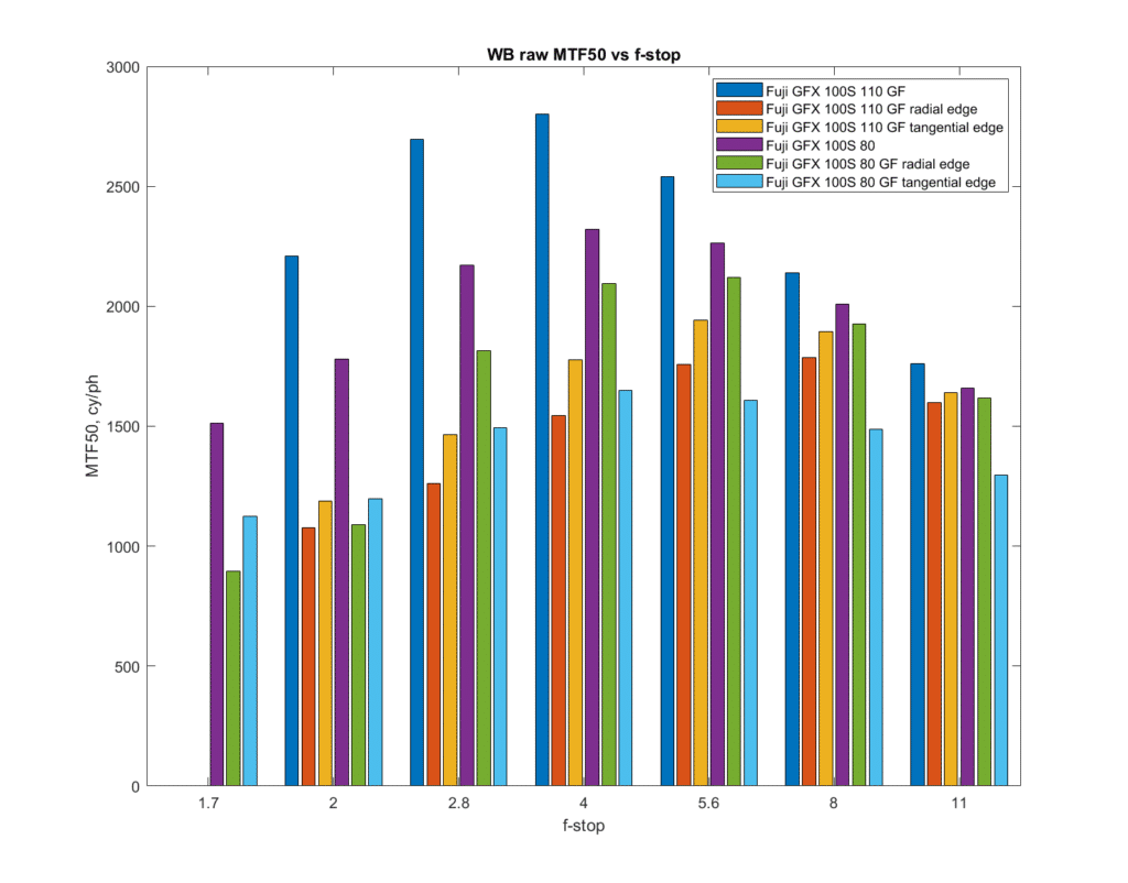
I measured the MTF50 on each of the raw channels, and am reporting on the MTF50 on a white-balanced composite of those channels, which is mostly the green channel. Wide open, the 110 GF is about half as sharp on the edge as it is in the center. The best compromise f-stop for the 80 seems to be f/5.6 or f/8.

The 80 just isn’t at sharp as the 110 in the center. But at f/2 through f/5.6 the off-axis sharpness appears to be about the same. At f/8 and f/11, the 80 suffers when tested with tangential edges.

Another way to look at sharpness is microcontrast, which is defined as the contrast at a particular frequency not far from Nyquist. I prefer 0.25 cycles per pixel.

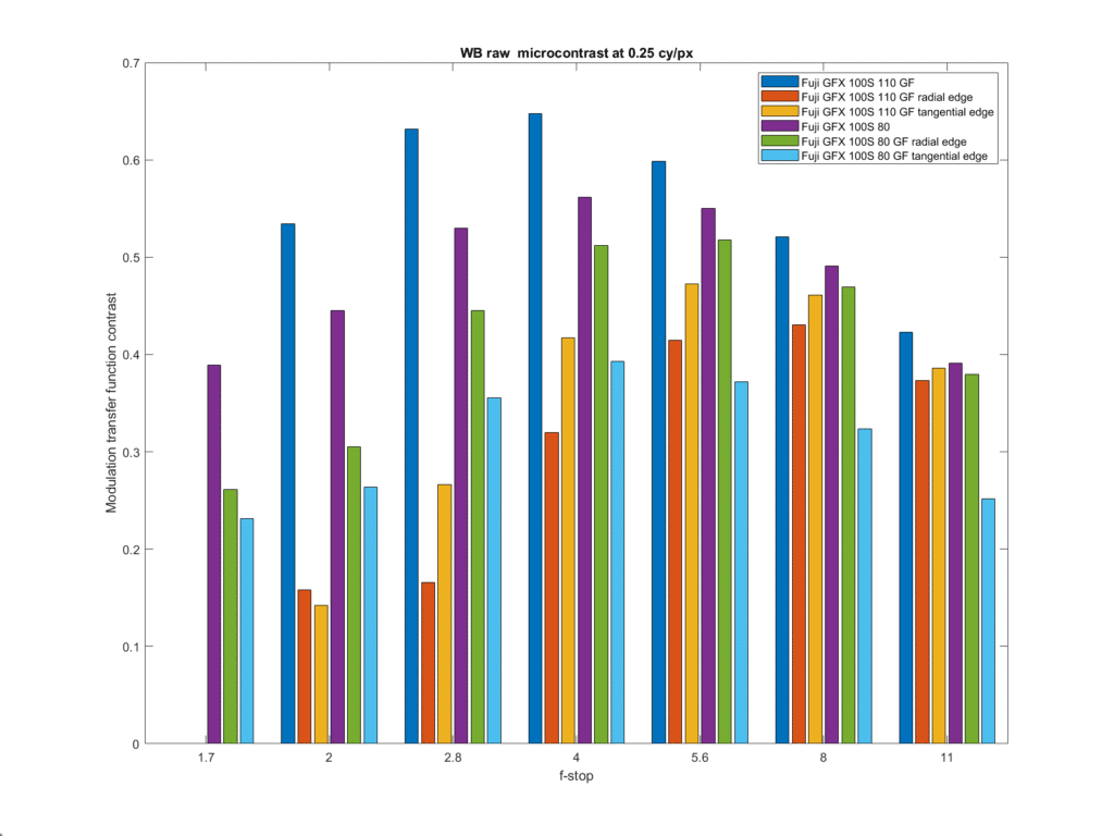
The 80 actually has better off-axis microcontrast than the 110at f/2 through f/4.

Some people use 0.33 cycles per pixel for microcontrast.

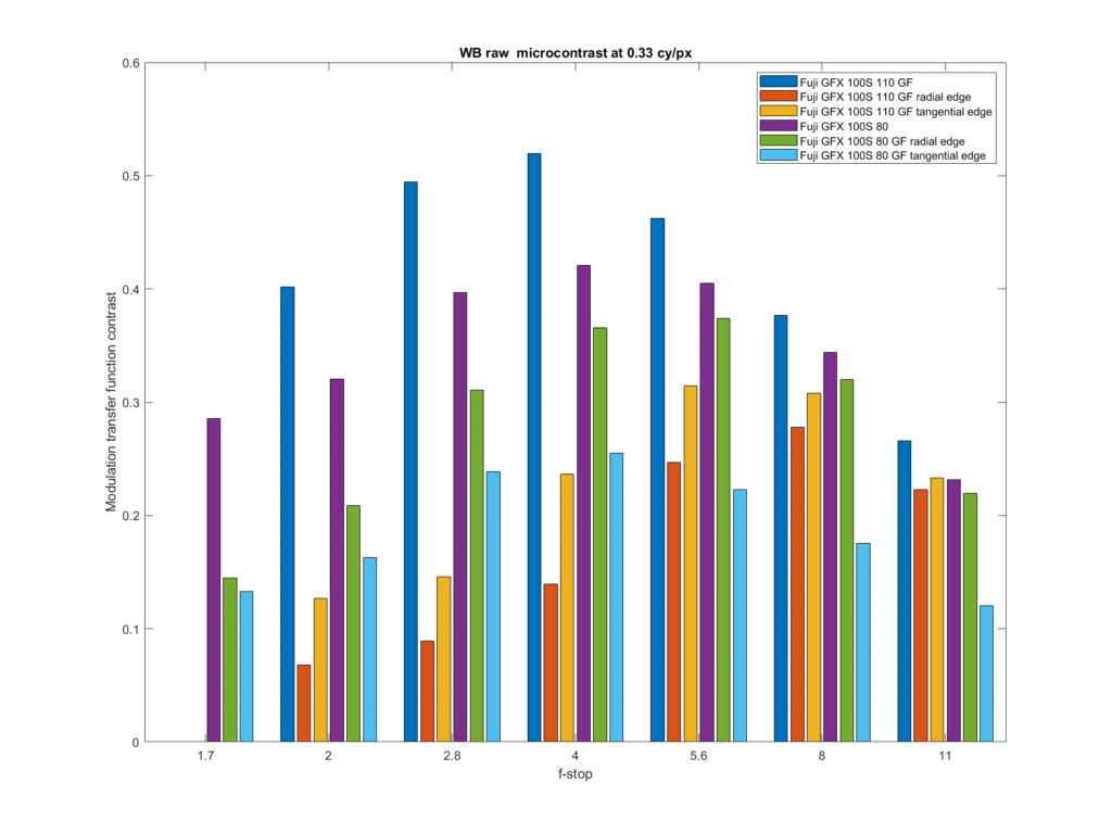
The numbers are worse, but the story is the same.

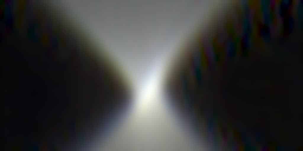
If you tell you you want to see the longitudinal chromatic aberration LoCA) numbers, I’ll show them to you, but I think the transfocal bokeh plots are more revealing, partly because they have more detail.

The vertical direction is the shift of the focal plane with respect to the plane of the sensor. Focus distance runs from top to bottom, with front-focused at the top and back-focused at the bottom. The horizontal axis a heavily-magnified view of distance in the sensor plane. The colors are highly approximate; I just assigned the raw channels to their respective sRGB channels. Almost all of the above presentation is front-focused because I didn’t set the distance properly.