• site home
  • blog home
  • galleries
  • contact
  • underwater
  • the bleeding edge

the last word

Photography meets digital computer technology. Photography wins -- most of the time.

You are here: Home / The Last Word / A single-pixel sensor model

A single-pixel sensor model

December 10, 2014 JimK Leave a Comment

In analyzing the photon transfer performance of a digital camera, it is usual to construct a model of the camera’s imaging properties, and then determine the parameters of these properties should the camera under test conformed to the model. It is also useful to know those areas for the camera does not work as the model says it should.

Here is the model that I’m using:

Digital Camera schematic

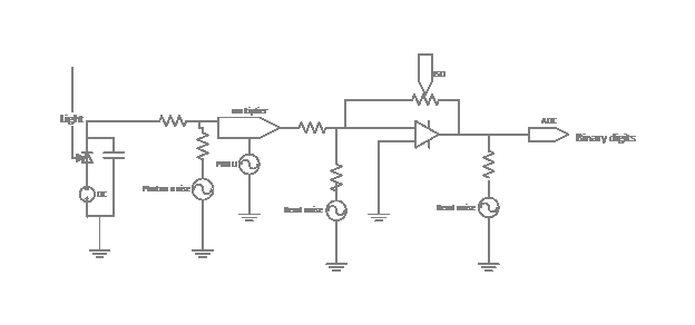
For the most part, this models a single pixel. There is one important deviation from that, and I’ll explain that when I get to it.

Let me walk you through the model.

Light falls on a back-biased photodiode, causing electrons to accumulate on the plate of a capacitor. Because of the physics of light, there is noise – called photon noise — associated with that process. You can consider the charge on the capacitor to be the sum of a DC – zero frequency – signal measured in electrons, and a Gaussian noise source whose standard deviation is the square root of the DC signal. This noise source, like all the others in the model, are sampled once per exposure.

The next noise source is photon response nonuniformity a.k.a. photo response nonuniformity, a.k.a. PRNU. Rather than adding to the DC signal, this can be thought of as multiplying it by a number whose mean is one and whose standard deviation is a measure of the PRNU. This is the part where the single pixel model breaks down, since PRNU is usually a fixed pattern error, and for any particular pixel, there is no noise. In fact, I would be happy to not consider it noise at all, but the convention is to do so, and in this instance I will go with conventional wisdom.

There is an amplifier between the capacitor and the analog-to-digital converter. The gain of the amplifier is determined by the ISO setting in the camera. There are a group of noise signals that don’t vary with the number of electrons on the capacitor. These signals are referred to collectively as readout noise, or simply read noise.

There are three ways to model read noise. The first is to measure it for each ISO setting as if it all occurred before the amplifier. In this case the units for read noise are electrons. The second way is to again measure it for each ISO setting, as if it all occurred after the amplifier. In this case the units are usually specified in terms of the least significant bit of the entity converter. The third way is to measure the noise at all ISO’s, compute the gain of the amplifier for each one, and calculate what must be the value of the preamplifier read noise and the post amplifier read noise. The Matlab model does the first and the third calculation.

The analog-to-digital converter is assumed to be perfect. To the degree that it is so, the quantization noise introduced by the ADC is part of the post amplification read noise. To the extent that the ADC introduces noise because of its imperfections this is also part of the post amplification read noise.

With the exception of PRNU, and any part of the read noise that doesn’t change from exposure to exposure, the single pixel model can be used to explain noise within a single image, by assuming that every pixel in the camera behaves identically, so the exposure to exposure noise of the single pixel model turns into variation among the pixels of a single capture.

Tomorrow: the sensor characterizer in action.

The Last Word

← Automatic sensor characterization, an introduction Sensor photon transfer analysis: PRNU →

Leave a Reply Cancel reply

Your email address will not be published. Required fields are marked *

May 2025
S M T W T F S
 123
45678910
11121314151617
18192021222324
25262728293031
« Apr    

Articles

  • About
    • Patents and papers about color
    • Who am I?
  • How to…
    • Backing up photographic images
    • How to change email providers
    • How to shoot slanted edge images for me
  • Lens screening testing
    • Equipment and Software
    • Examples
      • Bad and OK 200-600 at 600
      • Excellent 180-400 zoom
      • Fair 14-30mm zoom
      • Good 100-200 mm MF zoom
      • Good 100-400 zoom
      • Good 100mm lens on P1 P45+
      • Good 120mm MF lens
      • Good 18mm FF lens
      • Good 24-105 mm FF lens
      • Good 24-70 FF zoom
      • Good 35 mm FF lens
      • Good 35-70 MF lens
      • Good 60 mm lens on IQ3-100
      • Good 63 mm MF lens
      • Good 65 mm FF lens
      • Good 85 mm FF lens
      • Good and bad 25mm FF lenses
      • Good zoom at 24 mm
      • Marginal 18mm lens
      • Marginal 35mm FF lens
      • Mildly problematic 55 mm FF lens
      • OK 16-35mm zoom
      • OK 60mm lens on P1 P45+
      • OK Sony 600mm f/4
      • Pretty good 16-35 FF zoom
      • Pretty good 90mm FF lens
      • Problematic 400 mm FF lens
      • Tilted 20 mm f/1.8 FF lens
      • Tilted 30 mm MF lens
      • Tilted 50 mm FF lens
      • Two 15mm FF lenses
    • Found a problem – now what?
    • Goals for this test
    • Minimum target distances
      • MFT
      • APS-C
      • Full frame
      • Small medium format
    • Printable Siemens Star targets
    • Target size on sensor
      • MFT
      • APS-C
      • Full frame
      • Small medium format
    • Test instructions — postproduction
    • Test instructions — reading the images
    • Test instructions – capture
    • Theory of the test
    • What’s wrong with conventional lens screening?
  • Previsualization heresy
  • Privacy Policy
  • Recommended photographic web sites
  • Using in-camera histograms for ETTR
    • Acknowledgments
    • Why ETTR?
    • Normal in-camera histograms
    • Image processing for in-camera histograms
    • Making the in-camera histogram closely represent the raw histogram
    • Shortcuts to UniWB
    • Preparing for monitor-based UniWB
    • A one-step UniWB procedure
    • The math behind the one-step method
    • Iteration using Newton’s Method

Category List

Recent Comments

  • JimK on Goldilocks and the three flashes
  • DC Wedding Photographer on Goldilocks and the three flashes
  • Wedding Photographer in DC on The 16-Bit Fallacy: Why More Isn’t Always Better in Medium Format Cameras
  • JimK on Fujifilm GFX 100S II precision
  • Renjie Zhu on Fujifilm GFX 100S II precision
  • JimK on Fuji 20-35/4 landscape field curvature at 23mm vs 23/4 GF
  • Ivo de Man on Fuji 20-35/4 landscape field curvature at 23mm vs 23/4 GF
  • JimK on Fuji 20-35/4 landscape field curvature at 23mm vs 23/4 GF
  • JimK on Fuji 20-35/4 landscape field curvature at 23mm vs 23/4 GF
  • Ivo de Man on Fuji 20-35/4 landscape field curvature at 23mm vs 23/4 GF

Archives

Copyright © 2025 · Daily Dish Pro On Genesis Framework · WordPress · Log in

Unless otherwise noted, all images copyright Jim Kasson.