[Added March 17, 2014]
A reader posted a comment that you can see stating that there must be a systematic flaw in my simulation. He was right. Details are in the comments attached to this post. I fixed the error, and the results are reported at the bottom of this page.
[Now, on with the original post. Be sure to scroll down to the bottom for the corrected difference image and text.]
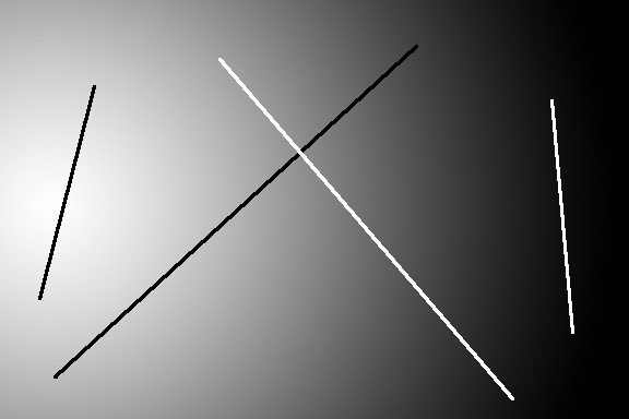
I created a synthetic image to stress the Sony raw compression/expansion algorithm. When I talk about companding in this post, I means the serial application of both halves of the algorithm. The image consists of a gradient, so that contouring should be readily apparent, and black and white lines, to force the differences between signals in a 32-column row to be large, and trip up the delta modulation part of the algorithm.
Here’s the test image:
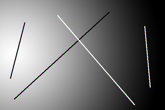
Here’s what it looks like after resampling with a RGGB Bayer CFA, passing through a 13-bit quantizer, and being demosaiced with bilinear interpolation:
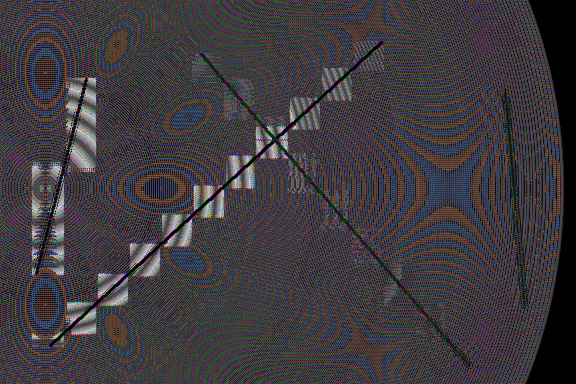
And here’s the difference (in Adobe RGB color space) between the 13-bit version, and the one that’s been companded: 13-to-11 bit tone compression, delta modulation and demodulation, and 11-to13-bit tone expansion, and then and being demosaiced with the same bilinear interpolation algorithm. I added an Exposure adjustment layer set to +10.0 so you can see the artifacts better:
- There is some strange moire in the gradient.
- There are 32-bit wide bands of added brightness around the black lines.
- There are similar, but less intense 32-bit wide bands around the diagonal white line.
This test is unrealistic in that there was no noise in the test image. Real captured images have photon and pixel response non-uniformity noise that can serve as dither to mitigate the visual effects of quantization errors, which is what we’re seeing here.
By the way, Lloyd Chambers has posted an image from one of his readers that shows similar artifacts in an actual a7R image.
[Now for the correction]
I computed the difference signal above in Photoshop by setting the blending mode of the compressed signal to Difference. As pointed out in the comments attached to this post, the original way I presented the difference image throws away all parts of that image where the companded image is brighter than the uncompanded one.
So this time I subtracted the demosaiced uncompressed image from the demosaiced compressed image in Matlab. I did this in a linear color space with the same primaries as Adobe RGB 1998, which is the color space I assumed for the camera native primaries. I know this isn’t the actual camera space, and I know that the 3×3 matrix multiply necessary to get from the raw RGB data to an approximation of Adobe RGB will have subtractions which can increase the visibility of any artifacts, but this is complicated enough as it is. Maybe later. Maybe much later.
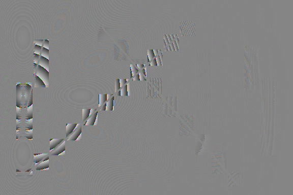
After I computed the error image with the subtraction in the previous paragraph, I biased the image so that the lowest pixel value was zero, and scaled the image into the range [0,1], noting the scale factor. Then I added the gamma of Adobe RGB, scaled to [0,16383], and wrote out the error image as a 16-bit TIFF. I read it into Photoshop, and exported it as a JPEG, which you see below.
The parts of the image with the smallest errors are the relatively featureless middle gray. The areas with positive errors are brighter than that, and the areas with negative errors are darker than that.
Also, the demosaicing of the uncompressed data in the original post was done with 8-bit precision, instead of 16-bit giving “errors” that were spurious, I fixed that as well, demosaicing both the uncompressed and the compressed images with 16-bit precision.
While I was messing around with the simulation, I converted it to use the latest breakpoints for the Sony tone compression curve that are published here.
In this model, the Sony ADC’s are assumed to be 14-bit, but you never see the effect of the last bit, because the steepest part of the tone curve has a slope of one half, resulting in every other histogram bucket being empty. Since provision is made for a 512-bit black point offset, the data actually spans a range of up to 16383 + 512 .
Because of the scaling, you can’t tell from looking at the error image how serious the error is. You need the scaling factor for that. For the image below, the scaling factor is 0.0551, meaning that the total span of the error is about 1/20 the span of the original image.
Ilya Zakharevich, the person who made the comments and got me back on the right track, feels that the artifacts observed by some people on real images are likely caused by rounding algorithms in the raw converter that are different from those employed by Sony in creating the compressed file. This is certainly possible. I may have not used the same rounding algorithm as Sony, but I used the same algorithm in both directions.
Ilya also believes that the right dither algorithm could improve the compression/expansion performance. I believe he’s right,


Hmm, your “with artefacts” zones are consistently brighter than those without. I suspect you used a wrong rounding function, so your model has a systematic error (proportional to the quantization step).
I suspect that without such a systematic error, the differences on your images would mostly disappear: 7 bit should be quite enough for (drop-noise dithered) images from a sensor with full well below 64K…
As stated in the post, I did the subtraction of the two images in Adobe RGB color space. Actually, I used the Photoshop difference layer blending mode to do the subtraction. That operation truncates the result at zero, and thus you can’t see the part of the difference that makes things darker.
So, there is a systematic error, but it’s not in the simulation; it’s in the way I processed the images for display on the web. To a first approximation, we are only looking at half the error.
Thank you for pointing this out.
I will rework the images by adding a bias signal, so that the correct value in the difference display isn’t zero, it’s a grey tone. Errors that increase luminance will be brighter than that grey tone and errors that decrease luminance will be darker. If that’s too confusing, I’ll consider generating an error image where no error is black and the absolute value of the error drives lighter values, but I hope I don’t have to do that, because we’re throwing away the sign of the error. I’ll work through this, and post an addendum to one or more of these posts soon.
Nice try, Jim!
However, I do not see any prevalence of black pixels in the image. If your explanation held water, about half of the pixels would be black.
I still think this is an indication of a bug. And I think that ALL the other yells of a “defect in Sony design” are just bugs in dequantizers. You see, to successfully dequantize, one MUST first know which of 5 possible rounding functions was used by the quantizer; otherwise you get a certain bias in your data. Such a bias is not a big deal if the quantization step is constant: then the bias is constant too, so it is just a shift in black level. Everybody knows how to deal with this.
However, if the quantization step is not constant, then your bias is different at different areas of the image. So everybody can see that your decoder is defective. (Of course, it is much more fun to bash Sony, so they would not say it is a bug in their raw converter…)
You are in a much luckier position than the rest of the guys: you have a source code of the quantizer, so you do not need to guess at the rounding function used. Good luck!
P.S. And remember: unless it is KNOWN in advance that the signal hitting the quantizer was “dithered enough”, a dequantizer also MUST dither by uniformly-distributed random noise in [-½,½] of quantization step! (Again, if the quantization step is constant, this may be done in post-processing; for variable quantization step, this MUST be done in the decompressor.)
“…I think that ALL the other yells of a “defect in Sony design” are just bugs in dequantizers. You see, to successfully dequantize, one MUST first know which of 5 possible rounding functions was used by the quantizer; otherwise you get a certain bias in your data. Such a bias is not a big deal if the quantization step is constant: then the bias is constant too, so it is just a shift in black level…However, if the quantization step is not constant, then your bias is different at different areas of the image.”
Ilya, are you saying that DCRAW and Rawdigger are decoding the Sony raw files improperly?
Jim
Ilya,
Good point about the number of black pixels. I am forced to consider that, in addition to the truncation of negative values in Ps, there is a systematic error in my algorithm, or, if my algorithm turns out to faithfully represent Sony’s, in the algorithm.
First off, let’s get the dither issue out of the way. While I recognize the desirability of dithering prior to quantization or requantization,
https://www.google.com/patents/US4187466
https://www.google.com/patents/US3999129
I didn’t add any dithering. I took my understanding of the algorithm from Alex Tutubalin and Lloyd Chambers, and I didn’t see anything about dither there. Do you know that Sony applies explicit dither? If so, can you tell me how they do it?
Now to the way I’m doing the tone compression and decompression. Here’s the Matlab code:
function self = compressTonesSony(self)

xVals = [0 1000 1600 2854 4058 8602];

yVals = [0 1000 1300 1613 1763 2047];

image13bits = round(self.normalizedImage * 8191);

self.toneCompressed = interp1(xVals,yVals,image13bits);

self.toneCompressed = round(self.toneCompressed);

end

function self = expandTonesSony(self)

yVals = [0 1000 1600 2854 4058 8602];

xVals = [0 1000 1300 1613 1763 2047];

expandedImage = interp1(xVals,yVals,self.deltaTranscoded);

expandedImage = round(expandedImage);

self.normalizedImage = expandedImage ./ 8191;

end
self.normalizedImage is in double-precision floating point, normalized to 1.0.
If you can see anything wrong, please let me know. I got the breakpoints of the interpolation curve from Alex’s tone curve lookup table. Notice that the top few hundred values on the interpolation curve will never be reached with a 13 bit encoding, which has confused me, but I figured it wouldn’t cause systematic errors since it’s symmetric for compression and decompresson.
I’ll be looking at this some more, thanks to your input, but if you can offer any help finding the error, I’d appreciate it.
And by the way, I don’t view what I’m doing as Sony-bashing. Doing this simulation work and finding how small the errors are has led me to have more confidence in the Sony compression algorithm, not less.
Jim
I tested the tone compression and expansion code by passing a 10000×10000 (100 megapixel) pixel image composed of uniformly distributed random double-precision floating point numbers through it. There is a mean error of 3.33964470181636e-05. Thus the image after the round trip thru the code is on average 30 parts per million brighter than the original image. The mean value of the difference image (after – before) is 3.33964486784473e-05, which is very close. The standard deviation of the difference image is 0.000421635110098892. The pixel with the maximum error has an error of 0.00103772429173121, and the pixel with the minimum error has an error of -0.00103772413988357. This seems reasonable.
However, when passing images quantized as 16-bit gamma-2.2 TIFFs through the simulation, there is a more significant gain in mean value than with the floating-point inputs. For the difficult test image, the “before” mean in linear, normalized-to-unity representation is 0.4620 and the “after” mean is 0.4632.
I found the error, or at least, an error. The demosaicing for the “before” image was being done with 8-bit depth, and that for the “after” with 16-bit depth. I’ll rerun the simulation, and post results.
When the error is fixed, the floating point and integer results are nearly identical. Also, the errors are much smaller.
Jim
This code is full of subtle biases (they might at the end cancel each other, I did not look) — but it is not the code which has the variable quantization step! This is analogue→11bit code, right?
One must analyse 11bit ↔7bit code instead.
“…it is not the code which has the variable quantization step! This is analogue→11bit code, right?”
This is the code that applies the tone curve to the 13-bit linear data and requantizes the data to 11 bit form (that’s the first method) and then reverses that operation (that’s the second method). Because of the nonlinear nature of the tone curve as specified in the xVals and yVals vectors, this provides quantization that is coarser at brighter 13-bit values than it is at dimmer ones.
The 11–>7–>11 bit transcoding operation is more complex (and I apologize for not being about to get the indenting formatted):
function self = deltaTranscodeSony(self)
self.deltaTranscoded = zeros(size(self.toneCompressed));
[rows,cols] = size(self.toneCompressed);
chunks = round(cols / 32);
for iRow = 1:rows
row = self.toneCompressed(iRow,:);
outRow = zeros(size(row));
for iChunk = 1:chunks
bottom = uint16((32 * iChunk) – 31);
top = bottom + 31;
chunk = row(bottom:top);
outChunk = zeros(size(chunk));
for j = 1:2 %once for even columns, once for odd
sampleIndex = uint16(j:2:(j+30));
sample = chunk(sampleIndex);
maxSample = max(sample);
minSample = min(sample);
span = maxSample – minSample;
if le(span,128)
step = 1;
else if le(span,256)
step = 2;
else if le(span,512)
step = 4;
else if le(span,1024)
step = 8;
else
step = 16;
end
end
end
end
for i = j:2:(j+30)
if eq(chunk(i),maxSample)
outChunk(i) = maxSample;
else if eq(chunk(i),minSample)
outChunk(i) = minSample;
else
diff = chunk(i) – minSample;
steps = round(diff / step);
outChunk(i) = minSample + (steps * step);
if gt(abs(chunk(i) – outChunk(i)),step)
halt
end
end
end
end
end
outRow(bottom:top) = outChunk;
end
self.deltaTranscoded(iRow,:) = outRow;
end
end
I do not think there is a need to read the source code. You have the wrongly decoded images, so you can guess the bias.
It looks like 0.0005 at the maximal-quantization-step case. So try to subtract const*quantization_step/max_quantization_step with const ≈ 0.0005, and redo the photon-dithered part. (Depending on what you subtract from what, the sign many need to be changed.) At some value of const, the bug should disappear.
But you need to have a correct difference image. Even with brain-damaged software, you can just Level one image to 128..255, Level another to 0..127, then take difference.
Ilya, I’m reworking all the code with the 512 count black bias and the 14-bit formulation in Alex’s post here:
http://www.rawdigger.com/howtouse/sony-craw-arw2-posterization-detection
Calling the ADC a 14-bit one seems a little silly since the slope of the steepest segment of Alex’s curve is 0.5, but I’ll play along. Including the black bias makes the effect of the tone curve more aggressive than the one I was using before.
I’ll post some results in the next few days, and I’ll put a comment here so you can see it. If you want to use the contact dialog box to send me you’re email address, I can contact you via email as well.
I’m now computing the difference in Matlab, as I should have been doing all along.
Thanks for your help on this.
Jim
About DCRAW:
when I read through its source code, I found several places where it is doing averaging like (a+b)>>1 (instead of the correct (a+b+1)>>1). So I know it DOES have bias (and does not decrease noise as far as it could) in certain areas. Why not in this one?
RAWDIGGER: do not know anything about it.
DITHERING in DEQUANTIZER: if 7-bit is enough (as it would be with:
• pure parabola in 13-bits-to-11-bits compression curve, and
• no-data-cooking pure-photon-noise sensor,
) then dithering is not needed.
However, we know that
• some cooking takes place (see my comment to http://blog.kasson.com/?p=3860#comment-134426);
• It is not a pure quadratic parabola.
Essentially: we do not know whether dithering is needed.
The correct dequantizing must include dithering; but most of the time, it is an overkill. (Quantizing is a noise reducer; if it reduces noise too much, one can see posterization; dithering AFTER dequantizing restores the original noise, and removes the defects. So one must see whether the noise is reduced “too much”.)
How to do dithering:: the simplest way to do it is:
• Assume that “8-bit is enough”, and do not dither these parts;
• So one must dither only in the areas where the quantization step is the maximal possible;
• So the dithering must be not “what is good for 7-bit”, but the convolution-quotient of “what is good for 7-bit” with “what is good for 8-bit”.
(This assumes that the end-user may add noise “needed for 8-bit regions” in post-processing — if they decide it is beneficial. Then in 7-bit regions, the dithering would be made “correct” too!)
Since convolution-divide of uniform in [-½,½] distribution by the uniform in [-¼,¼] distribution is point-masses at ±¼, the algorithm should be (4*data + random_plus_minus_1())*quater_quantization_step. (Or
((data<<2 + random_0_1()<> 2
Oups, my formula was cut-out by HTMLizer. Another try:
(((data<<2 + random_0_1()<<1 – 1)<<quantizer_exponent) + 2) >> 2
Yes, this is what is usually happens: integers in [0,1) (0 included, 1 not) are distributed very differently than floats in the same interval. 😉 To get the gist of what happens, you must use the same granularity as the actual data (for δ-compression, 11-bit input).
I think I need to be a little bit more explicit:
• Suppose you use floor() as your quantizer;
• Then the possible discrepancies are in [0,1);
• If you input is double, then the average of discrepancies (the bias) is ½;
• If your input is integer, then the bias is 0;
• If your input is half-integers, then the average discrepancy is the average of 0 and ½, so it is ¼;
• If your input is quoter-integers, then the average discrepancy is ⅜.
______________________________________________________________
On the third thought, maybe this distinction is just cutting the corners. If the input is integer, and the quantization step is a power of 2, then the bias of floor(data>>logstep) is going to be 0, ½, 1½,3½,7½ (for steps 1,2,4,8,16); so correcting for step/2 (as need for floating-point input) would have a bias -½, but that “remainder” bias is step-independent! Hmmmmm…
Jim, what the Rawdigger writes does not make a lot of sense:
Such a bold statement can be made only by Sony engineers, who know how the format is supposed to be decompressed. What Alex and Illiah have are just guesses. And their guesses are obviously wrong, since their images have larger bias in the parts of the image where the quantization steps are larger.
As I said in another comment, instead of
min_val + delta*step, I would trymin_val + (delta-0.5)*step.Ilya, I’m going to go ahead and nail down the simulated results based on Alex and Iliah’s work. Then, if I have the time and stamina, I’ll add some of your suggested refinements and see what happens. It sure would be nice if Sony told us exactly what’s going on.
Thanks,
Jim
I’m afraid we techies will never be able to understand possible legal ramifications of disclosures. Maybe they would be forced to disclose MORE stuff if they disclose ONE chunk?
An anonymous tip would not hurt, though! 😉
BTW, my email is everywhere on internet. Google for nospam-abuse()ilyaz. (And sorry, I thought the email I put in the header will be visible to YOU!)
Jim, thank you a lot for your rework of the tests! The new results look very interesting; moreover, it looks like there is no remaining bias of clearly-visible kind!
However, I must say that I have more remarks! 😉 ;-(
Your updated images are interesting, but, I’m afraid, may be a tiny bit misleading. First of all, you did not provide a “usual” passed-through-converter image, only a difference image.
Second, taking difference in linear space may provide a skewed result. For example, note that even after amplification, your image has practically no artifacts in the “near star trail” region (as opposed to “a wire on background of the sky” region). And the “near star trail” is the region the people find most troublesome! This may be due to the fact that the human vision does not operate linearly.
I trust that the CIECAM02 standard reflects the best knowledge about how human eye is sensitive to (difference of) “colors”. If my reading of the standard is correct, then
• With exception of painfully bright “colors”;
• and with exception of impossibly dark “colors”;
• and restricting attention to grayscale only;
the verdict is very simple: all you need to do is to compress the linear signal using γ=½. So I think the best result would be achieved by plotting
gray + amplification ×(√initial – √final).
If you use the same amplification factor as before (with signal normalized to [0,1]), your differences in bright region would decrease 2×, and differences in dark regions would increase a lot.
“Your updated images are interesting, but, I’m afraid, may be a tiny bit misleading. First of all, you did not provide a “usual” passed-through-converter image, only a difference image. ”
The before and after images look identical, and, because the web versions are JPEG’d, would fall apart under editing before the compression artifacts were visible.
Jim
Ilya Zakharevich seems to avoid discussing his own bias…
And that would be?
This conversation reminds me of graduate that is given the task of measuring the volume of a light bulb. With calipers and calculations he comes up with a + or – 3% estimate after hours of work. Within a matter of seconds, the taskmaster fills the bulb with water and then pours it into a graduated beaker to get the exact amount.
i.e. – Take photos of a gradient sky with a D810 and A7r and the same lens and then push and pull them to your desires. Way more often and way more readily Sony’s compression scheme will result in banding, posterization and artifacts than the Nikon file.
I’ve tried that with different results than you. That’s not an experiment that will expose the problems in delta mod part of Sony’s raw compression scheme; if the sky is pulled a lot, that will expose the coarseness of the tone curve part of the scheme.
Can you provide examples?
Jim
We’ve been in a rain pattern for months lately. Clear and gradient blue skies are a rarity lately. I have an idea though on how to make a test that can be duplicated by others and will see if I can do such a test in the next few days.
Thanks, Max.