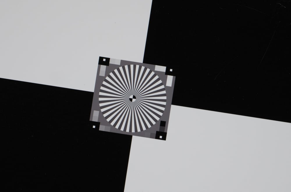
I do a lot of slanted edge MTF testing. It’s a very powerful technique. I use Imatest, MTFMapper, and occasionally Peter Burns’ Matlab code. Recently, on DPR, Frans van den Bergh posted a list of the assumptions behind the method. If you are interested in that technology, it’s worth a read. If not, this is going to be deep wading, and it’s probably best to past this post by.
Frans has allowed me to edit his DPR post for clarity and post it here as a guest post. All credit to him, and if there’s an error, it’s probably mine.
Frans’ assumptions:
1. The point spread function (PSF) is fixed over the region of interest (ROI) of the slanted edge (SE) method. We can improve our chances by keeping the ROI as small as possible (i.e., we limit the length of the ROI along the edge), but we have to balance this against noise, and having a long enough edge for oversampling to be effective.
2. The target object edge is actually straight (this is questionable for printed targets).
3. Following from assumptions 1 and 2, the edge intersects each photosite at the exact same angle. Since real-world sensor PSFs are not radially symmetrical, a violation of assumption 3 is similar to a violation of assumption 1 in that we end up averaging over slightly different PSFs along the edge.
4. The lens does not introduce any geometric distortion that would cause the image of the edge to deviate from a straight line. Of course, we can compensate for some curvature by modeling the edge as a curve instead of a straight line, but this runs the risk of violating assumption 3.
5. The angle of the edge with respect to the horizontal sensor axis (in the first quadrant) is such that oversampling is in fact achieved, hence the 5-degree edge angle guideline of the ISO 12233 standard. My quick-and-dirty version of this constraint would be that the dot product of the edge normal [-sin(theta), cos(theta)] and the photosite center locations [p, q] for all integers p and q must be such that
| |[-sin(theta), cos(theta)] . [p, q]| – 0.5| > d,
where d = 1/8 for 8x oversampling (or 1/4 for 4x oversampling). I have not yet figured out how to enumerate the angles theta for which the above equality does not hold, but some examples include theta in {0, 14.036, 26.565, 45} degrees.
6. The intensity values are linear (or have been converted to a linear representation).
7. The LSF decays rapidly enough in the across-the-edge direction relative to the width ROI so that the line spread function (LSF) is not truncated, or the modulation transfer function (MTF) measured by the SE method will actually be the convolution of the system MTF and sinc(f) (scaled to the ROI width).
8. The intensity values are free from clipping and saturation within the ROI.
9. The illumination within the ROI is uniform.
10. The edge orientation is estimated with sufficient accuracy. I think some of the earlier papers put the allowable error at 0.5 degrees, but I think that is too generous, and that edge orientation should be estimated to an accuracy of at least 0.1 degrees.
Thanks, Frans.

This is a nice list of the tall tentpoll gotchas. While not an assumption, another is that the MTF does not have nasty azimuthal minima not well sampled by the one or two edge orientations investigated.
For example, consider the imatest SFR or ISO 12233 test targets. They align (almost) with (x,y) over the full field of view. Now consider a well aligned lens – it has radial symmetry.
In the corner of the FoV, we expect there to be some coma, astigmatism, and lateral color. These are oriented along (tan,sag), which are (45,-45) degrees from (x,y). This means that the methodology of imatest or 12233 is completely blind to astigmatism, and does not sample “the worst” MTF coma or lateral color produces.
If you wish to evaluate a lens’ performance, it is best done with either MTF along (T,S), aligned with the axes, aberrations, and performance of the lens, or the azimuthal average. Sampling (T,S) and (x,y) are equally undersampled, azimuthally, but the samples are more badly chosen along (x,y) in the corners of the FOV. This produces an overestimate of the azimuthal average MTF in the corner, and does not at all produce an estimate of the (T,S) MTF there.
That is, IMO, no way to test a lens. It is also not a good estimate of the system performance, since the pixel’s worst MTF is also along (45,-45), so the underestimate is of the system performance in that orientation is even more severe.
For most users, lens testing is relative and not absolute. All of the extra math bs is inconsequential for a user (while important for an OEM) and how does this lens perform with this camera as a system is the answer they are looking for.
What’s important is consistency in testing so one can know that this lens copy is better than that lens copy or this lens is better than that lens. (resolution and symmetry)
After a while, one has known good sensors (flat and aligned), known good lenses (aligned) and a consistent process in photographing the test target.
I believe my results for the razor blade target are absolute, modulo the test conditions. Calling Frans’ list “math bs” means that you are not the person for whom I intended his post, and may mean that you are not the person for whom slanted edge testing is appropriate.
That “math bs” pays the bills, at least 🙂