I’ve given up on Photoshop for halftone processing of the firehouse images. I can’t see what I’m doing because the software that goes from file resolution to screen resolution has a bias in favor of black over white, so the images look darker than they should when the resolution is set so they fill the screen. If I zoom into 1:1, Photoshop does just fine displaying the pixels as they are in the image, but then I can’t see the overall effect. Lightroom displays the images approximately as they will print, but having to save the file and look at Lightroom every time I wanted to check on the effects of a change in settings was just too cumbersome.
In addition, Photoshop’s tools aren’t well suited to this kind of image manipulation. I couldn’t find a way to precisely move one of the two out-of-register images. I replaced the curves that went on top of the two image layers with a threshold layer, but I couldn’t set the threshold to fractions of an eight-bit value, even though the images were in 16-bit form.
Then I thought about what was numerically going on in Photoshop, and I realized that there was an important processing step that I wanted to control, but Photoshop wasn’t going to let my near it without some contortions.
So I decided to do the whole thing in Matlab.
First off, what am I doing in general? It’s easy to get a handle on the specifics, but I find that I’m better able to see the possibilities if I can clearly state the general case. I call what I’m doing autohalftoning. Halftoning is the process of going from a continuous image to a binary one. There are many ways to do halftoning, the two most popular being screens (once real, now universally simulated), and diffusion dither. In both cases, some high-spatial-frequency signal is added to the image to assist in the conversion of the information from 8- or 16-bit depth (contone) to 1-bit depth (binary). So the “auto” part of my made up word refers to using the high-frequency information in the image itself for dither. I’m not too proud to add noise if I need to, but so far, if I’m careful to stay away from the regions where the camera’s pattern noise is amplified, there seems to be no benefit.
In Photoshop, I offset two versions of the same image from each other by a small number of pixels, took the difference, and thresholded the result to get a binary image at the printer driver’s native resolution, which I then printed.
In Matlab to do an equivalent operation, I convolve the input image with a kernel that looks like this:
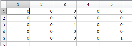
which performs the offsetting and the subtraction simultaneously. To simulate the way Photoshop computes differences, I truncate the negative parts of the image. That’s a pretty crude way to introduce what could be a subtle nonlinearity, so I’ve developed more sophisticate extensions of that basic approach; more on that in another post. Then I threshold the resultant image at a number that relates to the content of the output of the convolution operation, and that’s the binary image.
Here’s what you get with the kernel above:

It looks dull res’d down to screen size, but good coming out of the printer on a C-sized piece of paper.
The advantages of working in Matlab are
- Greater freedom in choosing the processing steps
- Greater control over those steps
- Perfect repeatability
- Speed
- Freedom from arbitrary bit depths; the interim images are all in double-precision floating point, and many of the processing variable are specified the same way.
- The ability to do automatic ring-arounds to observe the effect of multiple variable changes
- The ability to have the processing depend on the image content
Details to come.
Never heard someone mentions MATLAB and speed in the same sentence :-).
Probably not compared to optimized C++. Probably not compared to Python, either. There are many ways to write slow Matlab code; I usually find those ways when I first write an algorithm. Then I figure out how to change the 20% of the code that’s the bottleneck so that the whole thing runs fast enough. That means getting rid of for loops, if statements, and using Matlab’s tricky matrix indexing features. It also means getting rid of assignments to intermediate variables that I used in debugging to see what’s going on at each stage. All that makes the code less readable, at least to me. However, I have to admit that I’m starting to get used to it. A bit.
Matlab is quite good at self-parallelizing and using lots of cores if you don’t use constructs that force it into single-threading.
I guess fast is relative. For the things that I do in Matlab that have Photoshop sequences that perform the same algorithm, I find that Matlab is generally faster than Photoshop actions.
And if all else fails, there’s always the well-timed coffee break.
Jim
There’s another aspect of Matlab speed; the program’s rapacious appetite for memory. I run it mostly on a machine with 256 GB of RAM installed, and 192 GB addressable by Win 7. I’ve never seen it start to swap on that machine, but I occasionally did on a 48 GB machine I used to run it on, and when swapping it slowed to such a slow crawl that I always hit-C.
Jim