With the announcement of the Sony alpha 7S and its 12 megapixel sensor, the debate about the relative merits of big-sensel sensors and little-sensel sensors has heated up again. The two poles of the argument:
- Capture the image at as high a resolution as you can manage. If you need a lower-resolution version, you can downsample and average out all the extra noise that comes with the high-res image. If you need a high-res image, there’s no way you can res up a low-res one to get the same effect.
- There’s no substitute for a low-res capture if you don’t need any more resolution for your intended end use. Trying to res down a high res image will yield a noisier, artifact-filled result, and you’ll be sorry.
I thought maybe a simulation would be illuminating. I had the beginnings of what I needed from the camera simulation I used for the slanted edge MTF work. I added some code to allow the sim to take any target image and simulate an exposure with a camera whose characteristics I could choose.
Here’s what I chose:
- 10, 5, 2.5, and 1.25 um sensel pitch, with full well capacities (FWCs) of 160000, 40000, 10000, and 2500 electrons (e-).
- RGGB Bayer CFA with filters that are a diagonal 3×3 matrix multiply away from sRGB.
- Base ISO 100.
- Tested ISOs 100, 800, 3200
- Quantum efficiency 0.5
- Fill factor 1.
- Read noise: Gaussian with standard deviation 1.5 e- (favors larger pixels — all cameras are “ISOless”)
- Simulated Zeiss Otus at f/5.6. No distortion or any aberrations other than on-axis blur.
- Diffraction modeled at 450nm for the blue plane, 550 nm for the green planes, and 650 nm for the red plane.
- Demosaicing with bi-linear interpolation. No noise suppression. (favors larger pixels)
- Camera has a 14-bit, perfect ADC.
- No well saturation until clipping
- Zero pixel response non-uniformity (PRNU).
- No vibration or camera motion.
- With and without a 4-way beam-splitting antialiasing filter with a null at 0.67 of the sampling frequency, or 1.33 times the Nyquist frequency.
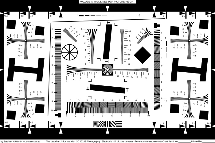
OK, that’s the camera. Next, I needed a target. Since one of the things to look at in the simulated captures is noise, I needed target images with as little of their own noise as possible. I picked two synthetic images. The ISO 12233 target is generated by a computer program (ignore the aliasing caused by downsampling the image for the web):
Bruce Lindbloom has produced a ray-traced image of an imaginary version of his desk:
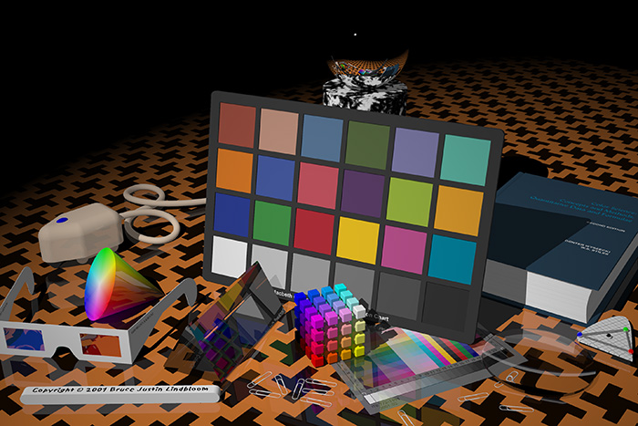
I used ETTR (and them some: 255/255/255 in the original maps to full scale) for the exposure for the Lindbloom image. This allow it to look good with no post-processing after demosaicing and conversion to sRGB. For the ISO 12233 target, I lowered the contrast so that it had the equivalent of a maximum sRGB value of 200/200/200 and a minimum of 55/55/55, to eliminate the possibility of clipping.
The next intellectual challenge was to find ways to compare the images from simulated cameras with different resolutions. To me, the most obvious two ways are to resample all the images to the resolution of the sensor with the finest pixel pitch (which might be important if you were thinking of making really big prints), resample all the images to the resolution of the sensor with the coarsest pixel pitch (which might be important if you were thinking of making small prints or high-res screen displays).
It’s clear that the algorithms chosen for the resampling will affect the results, so there’s another variable in the mix. There are a lot of moving parts here. Undaunted, I (maybe foolishly) waded into the project.
Here are the results for making big prints from the both target images. I have zipped up all the 16-bit TIFF files. There are 24 images in each file, one for each of three ISOs — 100, 800, and 3200 — four pitches — 10, 5, 2.5, and 1.25 um — and two possibilities for AA filter — with, and without. Although the files have no header, they are in the sRGB color space. These files are a bit over 200MB each. All the images therein are resampled to the resolution of the finest-pitch sensor in sRGB using Lanczos-3. There is reason to believe that that’s not the best way to resample these files, but that’s a work in progress.
http://www.kasson.com/ll/LindbloomTIFF.zip
http://www.kasson.com/ll/ISO12233TIFF.zip
For those of you who are willing to tolerate a bit of lossy compression, here are links to the same images as 8-bit sRGB JPEGs:
http://www.kasson.com/ll/LindbloomJPEG.zip
http://www.kasson.com/ll/ISO12233JPEG.zip
Some of my conclusions form the Lindbloom image:
The simulated Otus outresolves the 10-micron sensor by so much that, even with the AA filter, there are still obvious aliasing and Bayer artifacts. This is an ISO 100 image:
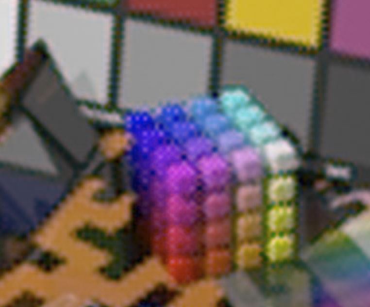
Even with the AA filter, there is still useful resolution improvement all the way to 1.25 micron, although the differences between 1.25 and 2,5 micron is not noticeable if you don’t pixel-peep.
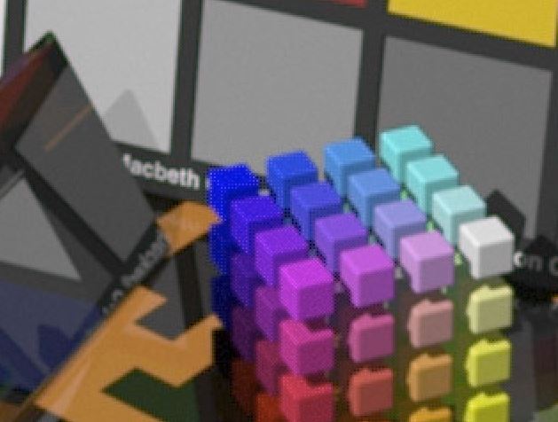
1.25 um ISO 100 with AA:
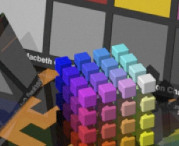
2.5 um ISO 100, With AA:
At ISO 3200, there’s a lot of noise at both the 1.25 and 2.5 micron pitches. Although some of that would be covered up by printer halftoning, it would probably make sense to sacrifice a little resolution.
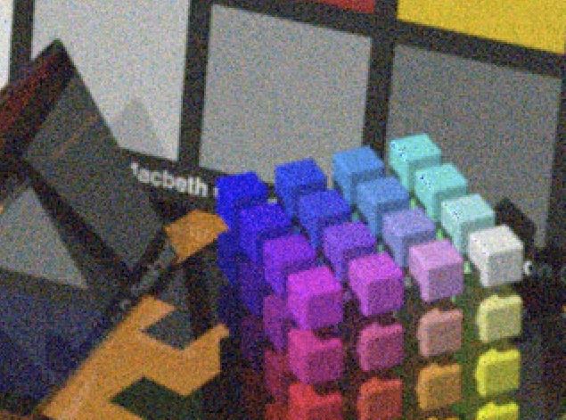
1.25 um ISO 3200, no AA:
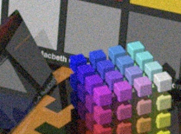
2.5 um ISO 3200 no AA:
At a 1.25 micron pitch, the AA filter does no good at all; the lens is performing enough antialiasing by itself. At 2.5 micron pitch, it’s not doing much. The AA filter does help a lot at 10 microns.
In general, the 10 micron pitch images look pretty bad. The simulated lens is way too sharp for the sensor. The 5 micron images look quite good. With some noise reduction, I think the 1.25 and 2.5 micron images would be the winners in all respects, but we’ll need more testing to confirm that.
Hi,
I just read the “executive summary” but I am notsurprised. I have seen some aliasing on 3.9 microns with my zoom lenses (ZA-series). So I would expect that 2-3 microns would be near optimal.
Thanks for your efforts!
Best regards
Erik