• site home
  • blog home
  • galleries
  • contact
  • underwater
  • the bleeding edge

the last word

Photography meets digital computer technology. Photography wins -- most of the time.

You are here: Home / The Last Word / Chromaticity Contrast Sensitivity Functions

Chromaticity Contrast Sensitivity Functions

April 28, 2014 JimK Leave a Comment

Yesterday, I presented material on how people’s ability to perceive small – and not so small – luminance changes varies with spatial frequency. Today, I’ll talk about how our ability to perceive changes in chromaticity (color without luminance) varies as spatial frequencies are manipulated. Yesterday, I started with the graphs and followed up with the visual demonstrations. Today, I’m going to reverse the order.

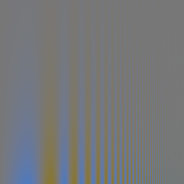
Exhibit A is an image that modulates between two CIELab values, 50,-35,0 and 50,35,0. Thus, L* and b* are held constant, and a* changes with a sinusoid that increases frequency exponentially (thus linear on log paper) from left to right, and reduces exponentially (thus linear on log paper) from bottom to top. If you back up a few feet and look at the places on the image where you can no longer make out the variations in color, you will get an idea of how your sensitivity to chromaticity changes along the a* axis varies with spatial frequency.

CSF visual1 lab a

Exhibit B is the same idea, but a* is 0 throughout, and b* is varied:

CSF visual1 lab b

In Exhibit C we go from one corner of the a*b* plane to the other:

CSF visual1 lab diag a

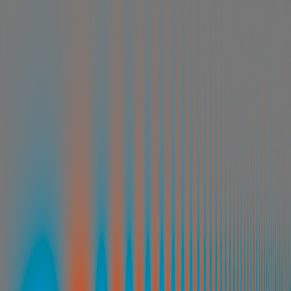
Exhibit D is the other diagonal:

CSF visual1 lab other diag

The sensitivity functions are not band-pass, as was the case yesterday with luminance. They are all low-pass, with the greatest sensitivity to change occurring at the lowest frequency. Not only that, but sensitivity falls more rapidly with increasing frequency than was the case with luminance changes.

In graphical form, with the luminance CSF curve for comparison, the chromatic CSF looks like this:

luma chroma CSF

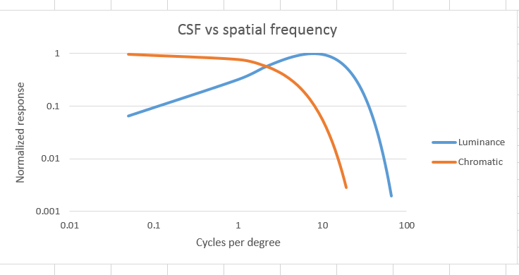
You can see that there’s no falloff in sensitivity for low spatial frequencies. You can also see that the lowpass falloff begins well before the luminance CSF peaks, and by the time that peak is over and the luminance CSF is starting to fall off with increasing spatial frequency, the chromatic CSF is way down there.

What’s that mean for photographers? We’ll look at that next time.

The Last Word

← Contrast sensitivity vs spatial frequency Contrast Sensitivity Functions and Photography →

Leave a Reply Cancel reply

Your email address will not be published. Required fields are marked *

May 2025
S M T W T F S
 123
45678910
11121314151617
18192021222324
25262728293031
« Apr    

Articles

  • About
    • Patents and papers about color
    • Who am I?
  • How to…
    • Backing up photographic images
    • How to change email providers
    • How to shoot slanted edge images for me
  • Lens screening testing
    • Equipment and Software
    • Examples
      • Bad and OK 200-600 at 600
      • Excellent 180-400 zoom
      • Fair 14-30mm zoom
      • Good 100-200 mm MF zoom
      • Good 100-400 zoom
      • Good 100mm lens on P1 P45+
      • Good 120mm MF lens
      • Good 18mm FF lens
      • Good 24-105 mm FF lens
      • Good 24-70 FF zoom
      • Good 35 mm FF lens
      • Good 35-70 MF lens
      • Good 60 mm lens on IQ3-100
      • Good 63 mm MF lens
      • Good 65 mm FF lens
      • Good 85 mm FF lens
      • Good and bad 25mm FF lenses
      • Good zoom at 24 mm
      • Marginal 18mm lens
      • Marginal 35mm FF lens
      • Mildly problematic 55 mm FF lens
      • OK 16-35mm zoom
      • OK 60mm lens on P1 P45+
      • OK Sony 600mm f/4
      • Pretty good 16-35 FF zoom
      • Pretty good 90mm FF lens
      • Problematic 400 mm FF lens
      • Tilted 20 mm f/1.8 FF lens
      • Tilted 30 mm MF lens
      • Tilted 50 mm FF lens
      • Two 15mm FF lenses
    • Found a problem – now what?
    • Goals for this test
    • Minimum target distances
      • MFT
      • APS-C
      • Full frame
      • Small medium format
    • Printable Siemens Star targets
    • Target size on sensor
      • MFT
      • APS-C
      • Full frame
      • Small medium format
    • Test instructions — postproduction
    • Test instructions — reading the images
    • Test instructions – capture
    • Theory of the test
    • What’s wrong with conventional lens screening?
  • Previsualization heresy
  • Privacy Policy
  • Recommended photographic web sites
  • Using in-camera histograms for ETTR
    • Acknowledgments
    • Why ETTR?
    • Normal in-camera histograms
    • Image processing for in-camera histograms
    • Making the in-camera histogram closely represent the raw histogram
    • Shortcuts to UniWB
    • Preparing for monitor-based UniWB
    • A one-step UniWB procedure
    • The math behind the one-step method
    • Iteration using Newton’s Method

Category List

Recent Comments

  • JimK on Calculating reach for wildlife photography
  • Geofrey on Calculating reach for wildlife photography
  • JimK on Calculating reach for wildlife photography
  • Geofrey on Calculating reach for wildlife photography
  • Javier Sanchez on The 16-Bit Fallacy: Why More Isn’t Always Better in Medium Format Cameras
  • Mike MacDonald on Your photograph looks like a painting?
  • Mike MacDonald on Your photograph looks like a painting?
  • bob lozano on The 16-Bit Fallacy: Why More Isn’t Always Better in Medium Format Cameras
  • JimK on Goldilocks and the three flashes
  • DC Wedding Photographer on Goldilocks and the three flashes

Archives

Copyright © 2025 · Daily Dish Pro On Genesis Framework · WordPress · Log in

Unless otherwise noted, all images copyright Jim Kasson.