We’ve seen that the sensitivity to luminance variation falls off as the luminance spatial frequency increases. If turns out that it also falls off as spatial frequency decreases, giving a band-pass filter effect, which sharpens edges, and gives rise to the Mach Banding that we’ve been looking at in the preceding posts. There are many ways that psychologists have used to quantify this effect. One test looks at people’s ability to detect changes in luminance at various spatial frequencies. A graph of the inverse of the minimum detectable contrast versus frequency is called a Contrast Sensitivity Function, or CSF.
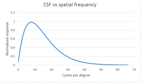
Here’s what a typical CSF looks like:
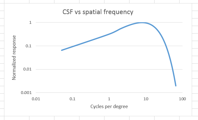
And here it is cast into the log-log plot that engineers usually employ to look at frequency responses:
There is a way that you can get a rough idea of your own CSF. Take a look at this picture from several feet away:

In the image, which I produced by writing Matlab code, the spatial frequency of the horizontal sine wave increases exponentially (or linearly on log paper) from left to right, and the amplitude of the sine wave deceases exponentially (or linearly on log paper) from bottom to top. If you find the right distance and look for the places where you can’t quite make out the sine wave, you can see a curve somewhat like the log-log one above. It’s not a perfect demonstration, especially at the lower frequencies where the phase of the sine wave artificially raises or lowers the contrast sensitivity, but I spent so much time programming it that I just have to show it to you.
I probably need to say a few words about the horizontal axis. We photographers talk about spatial frequency a lot, but we usually measure it in cycles per pixel, cycles per image height, line pairs per millimeter, or some such. How do we relate cycles per degree to those more-familiar units?
On capture, we can tie the units together by considering the angle of coverage of our lenses.
Let’s take the so-called normal lens for a 35mm, camera, the 50mm lens. It’s actually a bit longer than the usual definition of a normal lens, which is one whose focal length is the diagonal of the format. The 50mm lens on a 35mm camera has a horizontal angle of coverage of about 40 degrees. With a rectilinear lens and a flat subject, the periphery of the scene is mapped to the focal plane with a magnification that varies across the field. I’m going to ignore that; we’re just looking for an approximation here. The D800 and the a7R have horizontal resolutions of close to 8000 pixels, so each degree is about 200 pixels. Therefore, the highest spatial frequency that the camera can resolve is 100 cycles per degree (Nyquist says we need two samples per cycle).
Looking at the log-log CSF curve above, we can see that the human eye can’t resolve much of anything at 100 cycles per degree, so the camera is doing a better resolving job than a human could. 20/20 vision is 30 cycles per degree, and the maximum human resolution is about 50 cycles per degree.
In fact, even with a good 15mm lens, the camera’s going to be able to see details that a human wouldn’t be able to make out.
Well, that’s interesting, but not particularly actionable. On output, things get more interesting.
What resolution do we need in our prints so that the limiting factor is the eye of the observer? It depends on the viewing distance. From 1 foot 30 cycles per degree corresponds to about 180 micrometers. Since we need two pixels per cycle, we need more than 290 ppi to give the viewer all the information she can handle. Isn’t it convenient that Epsons print at 360 ppi and Canons at 300? That’s probably not a coincidence.
Using 300 ppi as our 30 cycles/degree measure, if we want our prints to hold up from a foot away, and we have a D800 with 7360 horizontal pixels, we can make prints 24.5 inches wide.
Now let’s consider where human peak contrast sensitivity occurs, at 10 cycles per degree. At one foot viewing distance, that’s about 540 micrometers, or half a millimeter. With our 300 ppi print, that’s six pixels. So, all you pixel peepers, if you see problems on your a7R or D800 images that are 4 or 5 pixels in extent, they’ll probably stick right out on a 24 inch wide print.
Leave a Reply