This is the fourth in a series of posts showing images that have been downsampled using several different algorithms
- Photoshop’s bilinear interpolation
- Ps bicubic sharper
- Lightroom export with no sharpening
- Lr export with Low, Standard, and High sharpening for glossy paper
- A complicated filter based on Elliptical Weighted Averaging (EWA), performed at two gammas and blended at two sharpening levels
The last algorithm is what I consider to be the state of the art in downsampling, although it is a work in progress. It’s implemented using a script that Bart van der Wolf wrote for ImageMagick, an image-manipulation program with resampling software written by Nicholas Robidoux and his associates.
This post using a Fuji demonstration image. This is the first target image that is actually photographic, in that it was captured by an actual, not a simulated, camera.
Here’s the whole target:
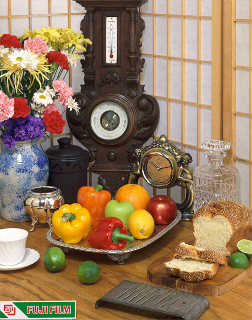
Now I’ll show you a series of images downsampled to 15% of the original linear dimensions with each of the algorithms under test, blown up again by a factor of 4 using nearest neighbor, with my comments under each image.

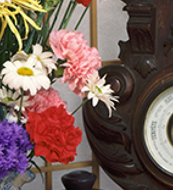
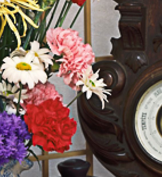
Bilinear interpolation, as implemented in Photoshop, is a first-do-no-harm downsizing method. It’s not the sharpest algorithm around, but it hardly ever bites you with in-your-face artifacts. That’s what we see here.
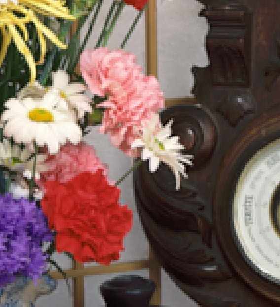
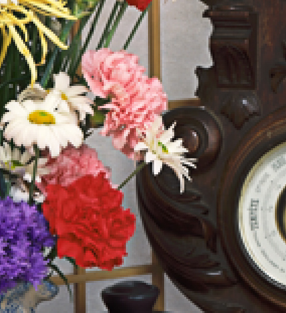
Photoshop’s implementation of bicubic sharper, on the other hand, is a risky proposition. Look at the halos around the flower stems, the flowers themselves, the clock, and just about everywhere.

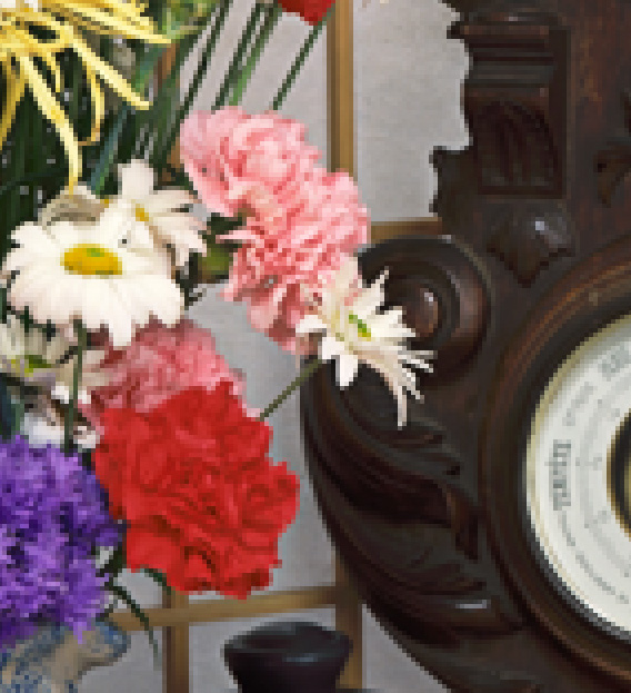
With the sharpening turned off, Lightroom’s export downsizing is, as usual, a credible performer. It’s a hair sharper than bilinear — though in this image the two are very close — and shows no halos, or any other artifacts that I can see.
I’ll skip over the various Lightroom sharpening options, and just include the images at the end. We’ve seen before that these don’t provide better performance than no sharpening when examined at the pixel-peeping level, although they might when printed.
For this crop, EWA looks a lot like Lightroom’s export processing, but with some lightening of the first third of the tone curve in high-spatial frequency areas. Look at the clock near the white flower, and the green stems near the yellow flower at the upper left corner.

Withe the deblur dialed up to 100, the image crisps up nicely. The downside is mild haloing around the clock and the stems.
In general, the differences with this scene are less striking than with the artificial targets used in previous posts.
Approaches that involve scaling then sharpening, based on a reduced set on information, seem fundamentally flawed to me (unless you are deliberately aiming to introduce halos to increase apparent sharpness). The sharpening is an attempt to recreate some of the detail you’ve just thrown away – why not just do a better job of selecting what information you keep and what you discard during the scaling process? ImageMagick gives you crude control over that selectivity with the filter:blur parameter.
I’ve found even a simple Gaussian downsample in ImageMagick comes pretty close to the performance of your EWA examples, with the right selection of blur factor. As far as I can tell ImageMagick’s Gaussian downsample is equivalent to Gaussian blur followed by “true” bilinear (i.e. nearest four neighbours) downsampling. The degree of blurring is controlled by the “-define filter:blur=” parameter, with 1.0 as the default. It operates as a convenient slider to trade off between softness and noise/moire/blockiness. I’ve had fairly good results with a value of 0.7, but the optimal value is going to depend on the source image and your intent/preference for the output. Here’s what I used on Bruce Lindbloom’s test image:
convert DeltaE_16bit_gamma2.2.tif -colorspace RGB -define filter:blur=0.7 -filter gaussian -resize 15% -filter point -resize 400% -colorspace sRGB foo.tiffThat’s what I was doing with Matlab’s imresize when I started this series. I did plot some noise reduction graphs here:
http://blog.kasson.com/?p=7101
but I never got around to looking at the spectra and comparing it to the other methods. I started out looking at downsizing algorithms with the idea of gaining some insight into the noise part of photographic equivalence theory. I’ve gone far enough down that road to be convinced that it’s valid. If you want to participate in working of perfecting downsampling, I suggest you head on over to this immense thread:
http://www.luminous-landscape.com/forum/index.php?topic=91754.0
and dive in.
I’ll be finishing this series up in a couple of days and moving on to some work on color space transforms. I may return to it if there’s some progress. You can be part of that if you like.
Thanks,
Jim
Thanks – it’s a fascinating thread, but for downsampling it seems like a case of severly diminishing returns. If you rate that complex EWA method a 10, then I reckon a simple Gaussian downsample with the right blur value comes in at around a 9 (with the advantage that it’s simple enough for me to completely understand, so it can never surprise me with unexpected artefacts).
Edward: TTBOMK, Gaussian with .7 deblur is quite moiré-prone given how blurry it is. Try downsampling the fly http://upload.wikimedia.org/wikipedia/commons/8/85/Calliphora_sp_Portrait.jpg.