In this post , I looked for drop offs in chromaticity in the octave or two before the highest image frequencies, and failed to find them. Some had hypothesized that such a drop would be a reason for the relative undersampling of chromatic versus achromatic information in the Bayer Color Filter Array (CFA). I did find that chromaticity changes, measured in CIELab, were smaller than luminance changes over broad spatial frequency ranges in the sample images, but this is more of an argument for sampling chromaticity with reduced resolution than it is for rolling off the effective sampling frequency in the highest octave of sampled chromatic spatial frequencies, like the Bayer CFA does.
However I will attempt, using the material that I’ve presented over the last few posts about the way that the human eye responds to luminance and chromaticity changes versus spatial frequency, to argue that the Bayer CFA’s color choices are sensible because of the way we see.
Let’s review the Bayer pattern. It looks like this:
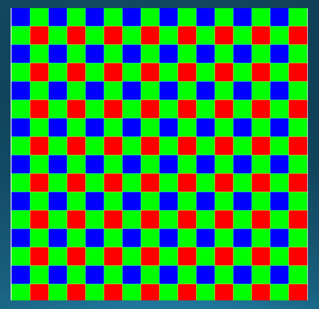
Of all the sensels, half respond to green light, a quarter to red, and a quarter to blue. The camera primaries are not sRGB. However, we can get a rough idea of how the various primaries contribute to luminance by looking at that color space. In sRGB, after linearizing, linear luminance (not the cube-rooted luminance in CIELab) is determined with the following equation:
Y = 0.2126R + 0.7152G + 0.0733B
The green component is almost three-quarters of the overall luminance. Thus, green can serve as a rough stand-in for luminance.
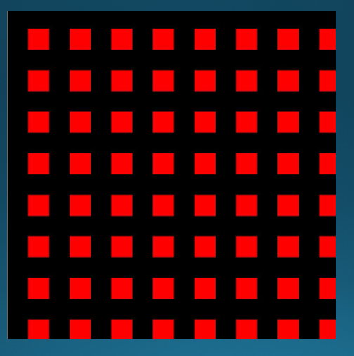
The pixels which are not sensed directly by the Bayer CFA must be generated in the demosaicing operation, either by interpolation from the sensels with that color filter, or from more complicated operations. Looking at just the green pattern of the Bayer CFA.

You can see that, except at the edges of the image, each blank in the green pattern is completely surrounded by green pixels that can be used for interpolation or other estimation.
Now, let’s look at the red pattern:
Some blank pixels have red sensels both above and below them. Interpolation using those squares will have half as much real-world data as in the case of the green pattern. In addition, there red pixels with no sensels at all above, below, to the right, or to the left of them. To interpolate information for these pixels, we need to look at the four sensels at the corners of the missing pixel. Now we have four sensels to use, as in the green case, but they are 1.4 times as far away.
Since the blue Bayer pattern is the red pattern shifted, everything in the paragraph above also applies to the blue pattern.
Interpolation is basically a lowpass function. Most of the other demosaicing techniques share that tendency. To the degree that most of the chromaticity information in the Bayer pattern resides in the red and blue portions of the pattern, the luminance component of an image reconstructed from will extend to higher spatial frequencies than those of the chromaticity components.
When the image is to be viewed by a human, any sizing aimed at producing the largest possible high-quality image will place the highest spatial frequencies of the luminance component on the steep slope to the right of the CSF curves. Along that whole slope, the chromaticity discrimination is almost two octaves worse than the luminance discrimination, so any loss in chromaticity resolution that stays within that amount won’t be noticed. The kinds of chromaticity resolution loss associated with demosaicing Bayer CFAs are at most a factor of two, or one octave, well within the safe region.
There are implications here for noise reduction. Performing noise reduction in general blurs the image. We don’t want to blur the luminance part of the image much, but, as we’ve seen, some blurring of the chromaticity parts will be invisible. The noise reduction tools in Lightroom and many other raw developers have separate controls for luminance and chrominance. It may look like you’re damaging the image if you pixel peep at a high magnification while manipulating the chrominance control, but, as long as the loss of chromaticity detail is only an octave or so from the level of luminance detail, you’re not hurting anything visible.
Do you have any intention of making a comparison between bayer CFA and Fuji’s “X-Trans” semi-random CFA?
I, for one, would find a technical breakdown and comparison of the two to be interesting.
(And just in case you’re not aware of what I’m referring to: http://en.wikipedia.org/wiki/Fujifilm_X-Pro1#Fujifilm_.22X-Trans.22_CMOS_sensor )