Dark Current in CMOS Sensors: Where It Comes From, and How Cooling Helps

In low-light or long-exposure photography, one of the most persistent sources of unwanted signal is dark current: thermally generated electrons that accumulate even in total darkness. Unlike read noise, which is largely constant from frame to frame, dark current grows with exposure time and varies from pixel to pixel.

Dark current is the rate at which thermal energy liberates electrons in the absence of light. These electrons are indistinguishable from photoelectrons, so they add a false signal that increases with integration time and contributes additional shot noise.

Sources of Dark Current in CMOS Sensors

Dark current arises from several physical mechanisms:

1. Thermal Generation in the Silicon Bulk

• Electrons are thermally excited across the band gap from the valence band to the conduction band.
• Dominant at moderate to high temperatures.
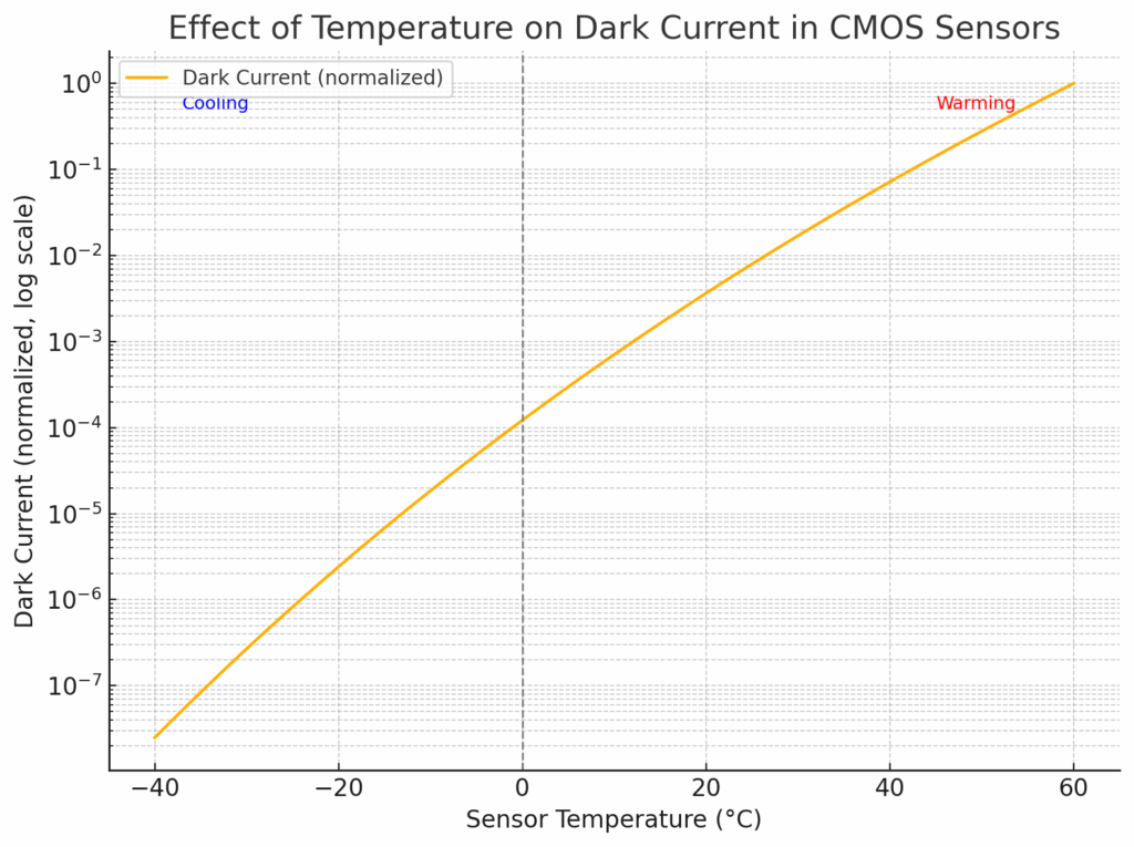
• Has strong temperature dependence:
  I_dark ∝ T³ × exp(−E_g / kT)
  where E_g is the band gap (~1.1 eV for silicon), k is Boltzmann’s constant, and T is temperature in Kelvin.

2. Generation at Surface States

• Imperfections at the Si-SiO₂ interface, often in the transfer gate region or at pixel edges.
• Surface traps can generate or release carriers.
• More prominent in older processes or poorly passivated sensors.
• Often shows strong pixel-to-pixel variation (a source of fixed pattern noise).

3. Edge Leakage and STI Defects

• Leakage currents along pixel boundaries or from shallow trench isolation (STI) defects.
• Found in small-pixel sensors with aggressive layout geometries.
• Often temperature-sensitive, but not always predictable.

4. Hot Pixels

• Pixels with unusually high dark current, often due to defects, dislocations, or contamination.
• Can be stable or develop over time due to radiation damage or thermal cycling.
• Often stand out more at higher temperatures and longer exposures.

Cooling primarily reduces thermal generation, which dominates bulk and surface dark current. Empirically:

• Dark current halves for every 5–7°C drop in temperature.
• This corresponds to the exponential dependence on 1/kT.
• Cooling from 25°C to –25°C can reduce dark current by ~30×.

This doesn’t just reduce false signal — it also reduces dark current shot noise, which follows:

σ_dark = sqrt(I_dark × t)

So as I_dark drops, the noise drops as the square root of the reduction.

Limits of Cooling

• Hot pixels may remain hot: Their leakage is often defect-driven, not thermally activated in the same way.
• Surface trap behavior is complex: Some states have long time constants or can generate bursts.
• Deep cooling (>–40°C) gives diminishing returns for most sensors unless you’re dealing with long integrations (e.g., astrophotography).

Best Practices

• Use thermoelectric cooling (TEC) to drop sensor temperature to a stable setpoint.
• Calibrate and subtract dark frames at each exposure time and temperature.
• Monitor hot pixel behavior over time; some may worsen with sensor age or radiation.

Dark current is a thermal problem at its core, and that makes mitigation possible. Cooling is by far the most effective strategy for reducing it, offering exponential improvements in signal fidelity for long exposures. For scientific and astrophotographic work, managing dark current is essential to approaching the theoretical noise limits of your sensor.