• site home
  • blog home
  • galleries
  • contact
  • underwater
  • the bleeding edge

the last word

Photography meets digital computer technology. Photography wins -- most of the time.

You are here: Home / The Last Word / Detectability of visual signals below the noise

Detectability of visual signals below the noise

September 17, 2017 JimK 14 Comments

I saw this pronouncement on DPR today:

The smallest signal we can distinguish from the noise floor is equal to the noise. Signal to noise ratio (SNR) = 1.

You see people saying that, or things very much like that, all the time. In some circles, it’s  conventional wisdom. 

There’s only one problem: it isn’t even close to being true.

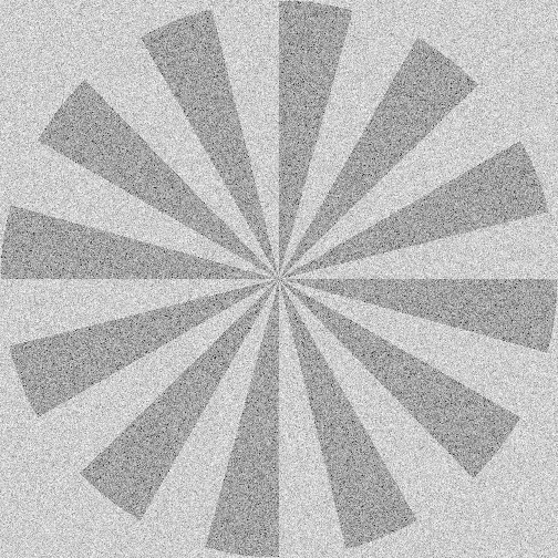
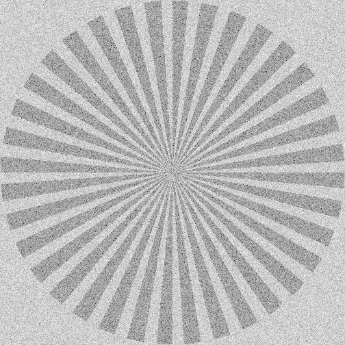
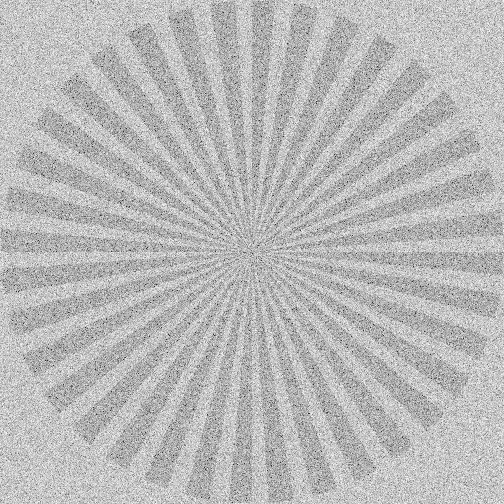
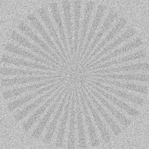
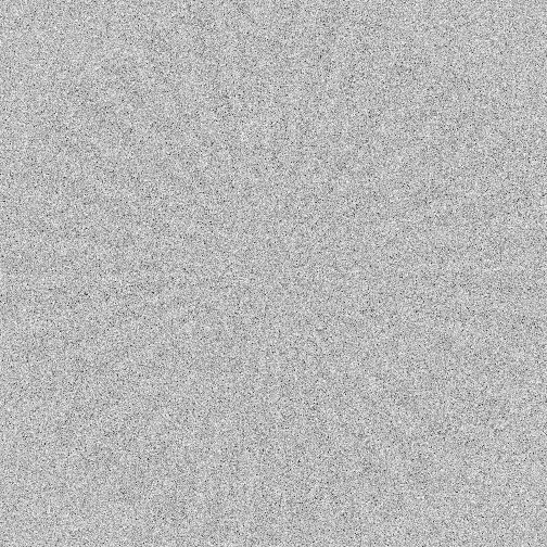
I’ve been meaning to post a demonstration for a while, and I spent the better part of half an hour coding up a program to make the images that I’m going to show you.

SNR = 2


SNR = 1


SNR = 0.5


SNR = 0.2


SNR = 0.1

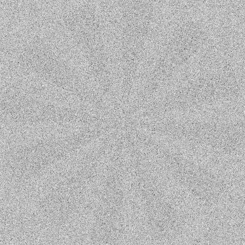
If you want to see the star better in the bottom image, try moving the image up and down with the scroll wheel on your mouse. 

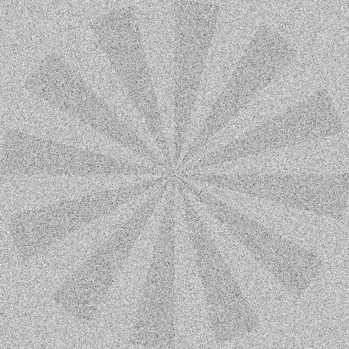
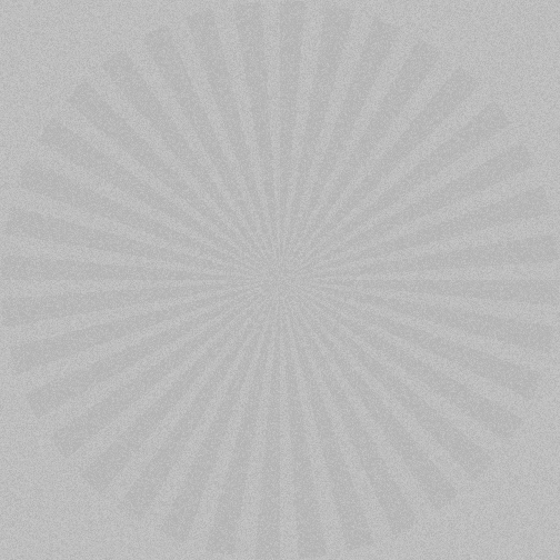
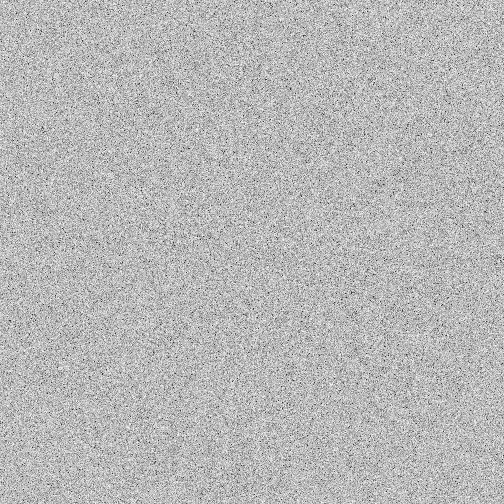
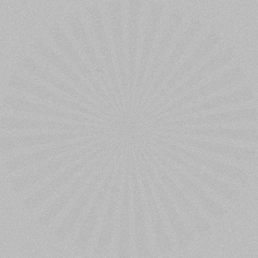
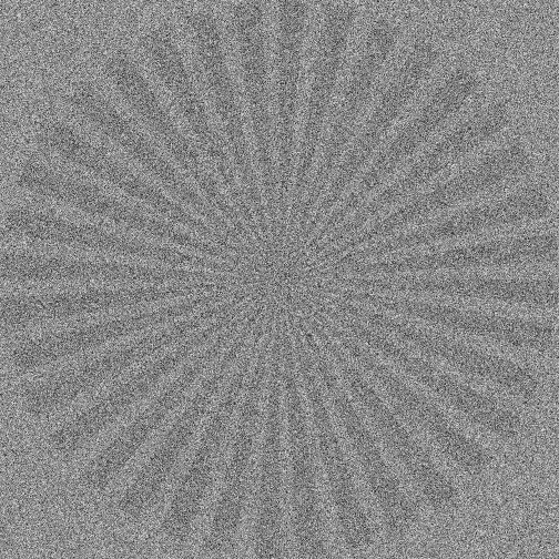
The noise is Gaussian, clipped at plus and minus three sigma. Mixing done in linear space. Images encoded for web at gamma 2.2.

You’ll notice that the parts of the star that are further away from the center are easier to distinguish when the noise gets high. That’s because there is more area for your eye to average over. 

If we look at images with more spokes to the star, this is easier to see:

SNR = 2


SNR = 1


SNR = 0.5


SNR = 0.2

A reader asked what happens if we average 24 frames with the above parameters. Here is the result:


SNR = 0.1

24 frames with those parameters average to:

If we take the above image and tighten up on the black and white points, we get this:

The Last Word

← Arca Swiss P0 Hybrid head Voigtlander 65/2 Apo Lanthar LoCA & focus shift →

Comments

  1. CarVac says

    September 17, 2017 at 5:45 pm

    For large scale detail, the SNR doesn’t have to be as high.

    The question is whether you can, say, read text of a given size at a given SNR.

    Reply
    • JimK says

      September 17, 2017 at 8:38 pm

      You are right on. With the Siemens Star stimulus, you can see the effect of raising the spatial frequency by looking closer to the center.

      Reply
    • JimK says

      September 18, 2017 at 12:49 pm

      I added another set of images that illustrates that better, with three times as many spokes.

      Reply
      • CarVac says

        September 18, 2017 at 4:36 pm

        It definitely makes it easier to see the point of extinction of the detail at the higher SNRs.

        Reply
  2. Herb Cunningham says

    September 18, 2017 at 9:01 am

    I am thoroughly convinced Jim needs to write a book of his wisdoms/tests for those of us who are even the slightest bit nerdy. Great stuff, Jim!

    Reply
  3. AndrewZ says

    September 19, 2017 at 2:01 am

    This is the same as audio. One would think that with 16 bits of resolution that you can only get 96db of dynamic range but with dithering of the last bit you can get at least another 12db. In fact with noise shaping you can extend it further with low frequency sounds as you have more sample points to play with (much like the wider spokes of the Siemens star). This is also quite common in the video world where you often have cameras claiming a dynamic range higher than the bit depth of the sensor as the same effect you have demonstrated above allows more values of grey to be filmed.

    Reply
  4. Eric Calabros says

    September 22, 2017 at 9:13 am

    Would be nice to see temporal noise reduction improvement applied to at least 24 frames of SNR 0.2 image.

    Reply
    • JimK says

      September 22, 2017 at 9:37 am

      I added that and a couple of more images to the bottom of the post. Thanks for the idea.

      Reply
  5. Graham Byrnes says

    September 25, 2017 at 11:49 am

    Just a comment from a (bio-)statistician: SNR is of course related to the r² metric (proportion of variance explained) in a regression. If we stopped at SNR=1 (r²=0.5) biomedical research would pretty much stop overnight 🙂

    Reply
  6. Vincent Wan says

    September 26, 2017 at 8:51 am

    Great post.
    The demonstration of the SNR .1 after averaging and contrast enhancement is impressive.

    Reply
  7. Eliz says

    November 22, 2017 at 1:04 am

    I’ve been thinking about this few days ago and now I see your article.
    Usually the electronic dynamic range is calculated with SNR=1 because many peoples consider you cannot distinguish source from noise once SNR becoming subunitar.

    But I personally imagined you actually can, because I remembered what I have read in this 2007 article:
    http://theory.uchicago.edu/~ejm/pix/20d/tests/noise/#patternnoise
    “Because the human eye is adapted to perceive patterns, this pattern or banding noise can be visually more apparent than white noise, even if it comprises a smaller contribution to the overall noise”
    So the ability of our brain to detect form shapes make us still see images when SNR<1.

    You can clearly see this in your test.

    Reply
  8. Bill Claff says

    January 19, 2021 at 1:55 pm

    What is implied in the pronouncement is detectable over black.
    In other words, the smallest “detectable” signal.
    If your test has used a black background and a star with SNR < 1 over that black I think the results would be different.

    Reply
    • JimK says

      January 19, 2021 at 8:56 pm

      Are you saying clip the noise at the mean and plus three sigma instead of plus and minus three sigma? If so, how would you expect the result to change?

      Reply

Trackbacks

  1. Detectability of visual signals below the noise, part 2 says:
    September 27, 2017 at 2:58 pm

    […] few days ago, I made this post about the visual detectability of information with a signal to noise ratio (SNR) of less than one. […]

    Reply

Leave a Reply Cancel reply

Your email address will not be published. Required fields are marked *

May 2025
S M T W T F S
 123
45678910
11121314151617
18192021222324
25262728293031
« Apr    

Articles

  • About
    • Patents and papers about color
    • Who am I?
  • How to…
    • Backing up photographic images
    • How to change email providers
    • How to shoot slanted edge images for me
  • Lens screening testing
    • Equipment and Software
    • Examples
      • Bad and OK 200-600 at 600
      • Excellent 180-400 zoom
      • Fair 14-30mm zoom
      • Good 100-200 mm MF zoom
      • Good 100-400 zoom
      • Good 100mm lens on P1 P45+
      • Good 120mm MF lens
      • Good 18mm FF lens
      • Good 24-105 mm FF lens
      • Good 24-70 FF zoom
      • Good 35 mm FF lens
      • Good 35-70 MF lens
      • Good 60 mm lens on IQ3-100
      • Good 63 mm MF lens
      • Good 65 mm FF lens
      • Good 85 mm FF lens
      • Good and bad 25mm FF lenses
      • Good zoom at 24 mm
      • Marginal 18mm lens
      • Marginal 35mm FF lens
      • Mildly problematic 55 mm FF lens
      • OK 16-35mm zoom
      • OK 60mm lens on P1 P45+
      • OK Sony 600mm f/4
      • Pretty good 16-35 FF zoom
      • Pretty good 90mm FF lens
      • Problematic 400 mm FF lens
      • Tilted 20 mm f/1.8 FF lens
      • Tilted 30 mm MF lens
      • Tilted 50 mm FF lens
      • Two 15mm FF lenses
    • Found a problem – now what?
    • Goals for this test
    • Minimum target distances
      • MFT
      • APS-C
      • Full frame
      • Small medium format
    • Printable Siemens Star targets
    • Target size on sensor
      • MFT
      • APS-C
      • Full frame
      • Small medium format
    • Test instructions — postproduction
    • Test instructions — reading the images
    • Test instructions – capture
    • Theory of the test
    • What’s wrong with conventional lens screening?
  • Previsualization heresy
  • Privacy Policy
  • Recommended photographic web sites
  • Using in-camera histograms for ETTR
    • Acknowledgments
    • Why ETTR?
    • Normal in-camera histograms
    • Image processing for in-camera histograms
    • Making the in-camera histogram closely represent the raw histogram
    • Shortcuts to UniWB
    • Preparing for monitor-based UniWB
    • A one-step UniWB procedure
    • The math behind the one-step method
    • Iteration using Newton’s Method

Category List

Recent Comments

  • JimK on Goldilocks and the three flashes
  • DC Wedding Photographer on Goldilocks and the three flashes
  • Wedding Photographer in DC on The 16-Bit Fallacy: Why More Isn’t Always Better in Medium Format Cameras
  • JimK on Fujifilm GFX 100S II precision
  • Renjie Zhu on Fujifilm GFX 100S II precision
  • JimK on Fuji 20-35/4 landscape field curvature at 23mm vs 23/4 GF
  • Ivo de Man on Fuji 20-35/4 landscape field curvature at 23mm vs 23/4 GF
  • JimK on Fuji 20-35/4 landscape field curvature at 23mm vs 23/4 GF
  • JimK on Fuji 20-35/4 landscape field curvature at 23mm vs 23/4 GF
  • Ivo de Man on Fuji 20-35/4 landscape field curvature at 23mm vs 23/4 GF

Archives

Copyright © 2025 · Daily Dish Pro On Genesis Framework · WordPress · Log in

Unless otherwise noted, all images copyright Jim Kasson.