This is a continuation of the development of a simple, relatively foolproof, astigmatism, field curvature, and field tilt test for lens screening. The first post is here.
Warning: this is a nerdy little post. don’t know how to interpret it myself. Maybe some of you do. If the words Fourier transform mean little to you, it’s probably a good idea to move on.
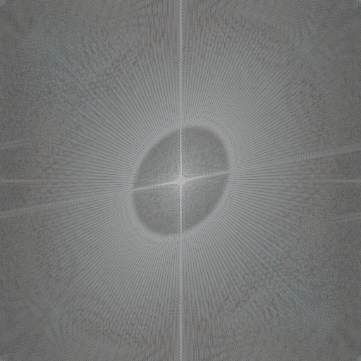
In this post, I showed the center, edge and corner renderings of a Siemens Star captured with a Sony 12-24 mm f/4 lens on a Sony a7RII. A couple of people wondered what the Fourier transform of the images that I posted there would look like. With the aid of Brandon Dube, I wrote this Matlab code:
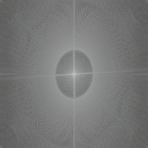
I exported the files from Lightroom, passed them through the above code, and this is what resulted for the lens set at 24 mm:

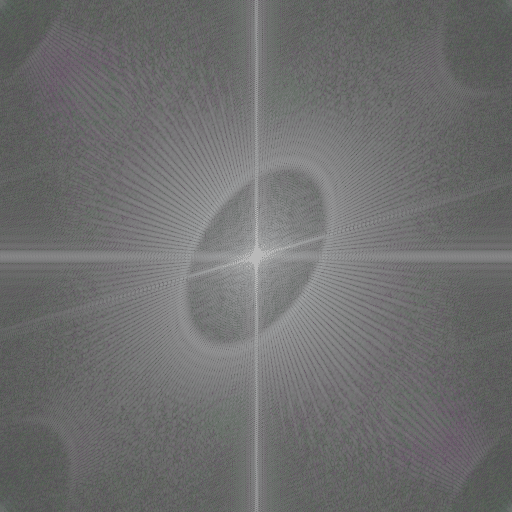


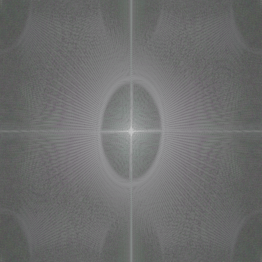


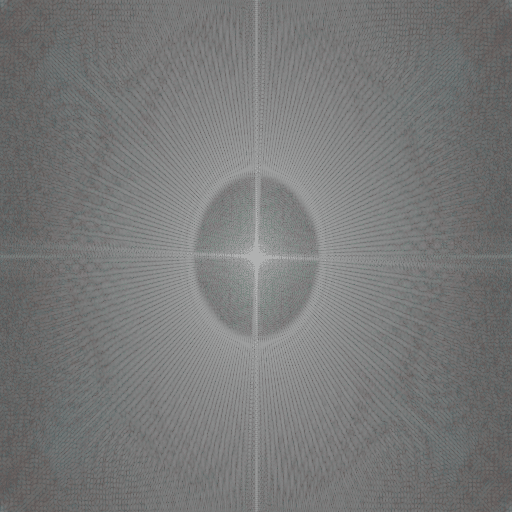
And at 18 mm:
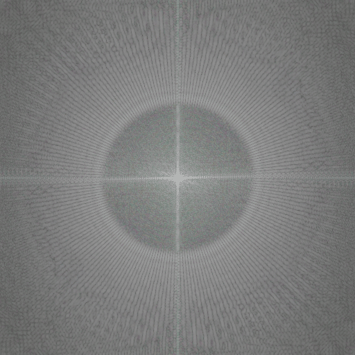

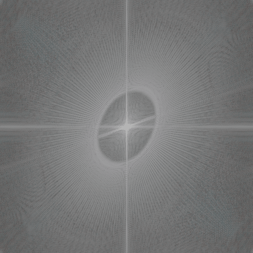

At 12 mm:
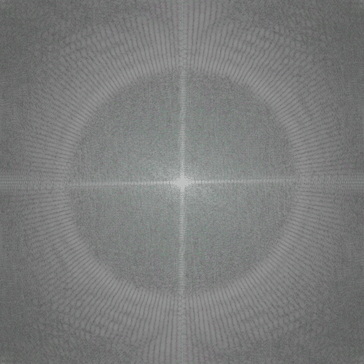

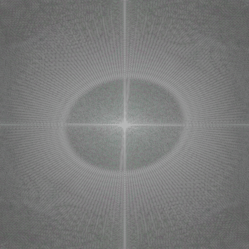

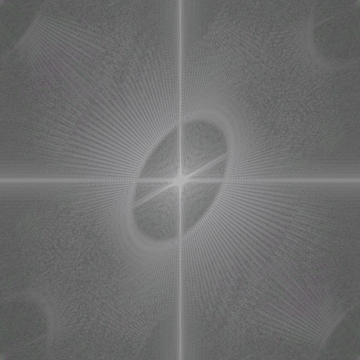

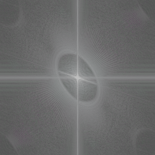
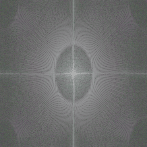
The images seem by and large well behaved, without obvious aberration.
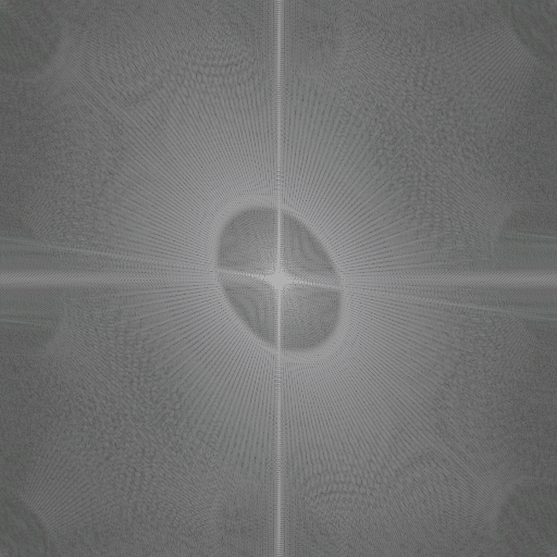
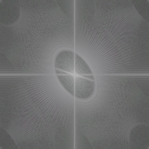
Ones like this: http://blog.kasson.com/the-last-word/fourier-sony-12-24-siemens-star/attachment/a7rii12-24at18-4fft/ have features jutting in from the edges. Those are aliasing. The holes in some of them are… I don’t know what. Maybe demosaicing related? The X/Y cross are related to the boundary of the image; if you pad with the value at the edges, it will go away. The other lines are related to the cross itself. The black hole is because of the phase inversion/lack of resolved-ness in the middle.
I think one method to acquire a truth so you can probe at the MTF is to take captures that are focused for best performance in the corners at like f/22, pull a raw color plane and interpolate it (or try one of the techniques available to compute its FFT when missing samples), then apply a filter (sharpen) in the fourier domain to pull the diffraction out of the image. This would allow you to poke at what aberrations are there more robustly in fourier space, where things are more separable.
The tape in the source images probably doesn’t help, it might be useful to write some object detection code to find the tape and paint over it with white in software.
Cheers,
Brandon
On second thought, the circular cutouts in the corners appear to be the result of distortion. I believe the central gray ring changing size is because the magnification is different, and lower, in the corners which means there is more high spatial frequency content.
I don’t know why the middle gray ring exists. Maybe it is because of the artifact (loss of contrast and inversion) in the center of your stars, or it is because they extend to the edge of the ROI.
If by the circular cutouts in the corners (and at the cardinal points) you mean the relative baseband images – those are due to aliasing, as baseband information is modulated out at cycles/pitch spacing by the pixel Bayer pattern (search for Dubois’ papers on frequency domain demosaicing). The chrominace information thus corrupts otherwise pristine grayscale information.
As for the baseband ‘ring’, I always thought that it was due to the fact that the star’s image represents a finite set of frequencies which terminate abruptly at the low end, below which there is suddenly relatively little energy and some noise. So the radius of the ‘middle gray ring’ should indicate the linear spatial frequency at the rim of the star.
Jack
I do not think the circular cutouts are to do with aliasing. If they were, they would appear (and be most severe) on axis where the lens will have its greatest resolution, since the camera contribution is (more or less) constant over the field.
Who says? You are thinking monochrome, this is Bayer.
Look up Dubois, it’s all there.
I read Dubois, “Frequency-Domain Methods for Demosaicking
of Bayer-Sampled Color Images” Dec. 2005. It does not seem to support your view. The crux of what I read from the paper is that the author proposes that for an aliased image, the aliasing has a directional preference, and the spatially localized weighting coefficients can be chosen separately for f_x and f_y (or pick two orthogonal angles) to best preserve the structure of the truth and suppress aliasing.
Ah, an idea.
To see what is related to demosaicing and what isn’t, try generating white noise and taking a picture of it. It contains all frequencies at all angles, so on-axis where the lens is diffraction limited (at least ish) and the pixel contribution is idealistic, you’re left with just the demosaicing-related component of the FT. (Some would object to calling it a transfer function, I do not)
Hi Jim,
Not that it will make a big difference, but the standard way to show these graphs is
freq = log(1+freq)/max(freq(:))); % from section 3.2 of G&W DIP
What is your objective in producing the 2D spectra? My experience is that they are really hard to interpret visually unless one knows specifically what they are looking for because of very poor discrimination in the z axis, which arbitrarily emphasizes low energy features (i.e. ^0.2 or log).
Jack
PS Also as you know my preference for these tests off neutral subjects is not to demosaic at all – and instead simply white balance the raw data. That takes one typically non-linear variable off the table when trying to estimate relative hardware performance.
My motivation in looking at the Fourier plots was to see if the type of lens aberration would be more obvious than with the straight photos. Brandon has sent me some synthetic images with various aberrations, which I haven’t posted yet. I’m still not convince that the FT stuff is helpful, but will probably mess with it some more.
As to the demosacied images, before I got sidetracked down this FT rabbit hole (to mix railroading and mathematician-turned-writer metaphors), my objective in this test was to come up with something that would be fairly easy for most folks to do without a lot of learning to use unfamiliar software.