For some time now, I’ve been analysing dark field photographs in the frequency domain for clues to whether or not cameras are applying spatial filtering to their raw files. I started when I was investigating why the Sony a7S suddenly had a better engineering dynamic range (EDR) when the ISO knob was turned from 50000 to 64000. One would think that, as ISO goes up, EDR would go down. The kink in the a7S EDR curve was puzzling. I participated in a discussion on DPR, and started to use some Matlab code supplied by a forum participant known as DSPographer to look at dark-field noise in the frequency domain.
Why dark-field noise? Because, in the absence of fixed pattern read noise (FPN), it contains equal energy per unit bandwidth — engineers say that it is “white”. And it turns out that most FPN is concentrated at frequencies much lower than the ones that camera manufacturers suppress in their efforts to use digital signal processing (DSP) to reduce noise levels.
Why the frequency domain? Because it’s easy to see the deviations from flat frequency response, and thus the tell tale signs of raw file cooking.
I have modified DSPographer’s code a great deal in the time that I’ve been using it, but the ides behind what it does is still the same: it gives the average frequency response of the power of a square image horizontally and vertically. Because we’re analysing noise, the frequency response is noisy. The code allows the averaging into frequency “buckets” to be adjusted. Many small buckets gives a fine-grained look at the power vs frequency, but the downside is more noise. I tend to us small buckets and let my eye do the averaging.
How does this frequency domain measurement deal with various kinds of sensor defects and post-processing? That’s the topic that I want to deal with in this and the next post. In this one, I’ll talk mostly about the defects.
In order to get at the effects of various defects, I built a little camera simulator in Matlab, and asked it to spit out raw color planes for Fourier analysis. One color plane is sufficient for this work, since for real cameras I analysis the raw planes one at at time. I set the camera’s precision to 14 bits, its base ISO to 100, its unity gain ISO to 320 (implying a full well capacity of about 45,000 electrons). I set the pre-amplification noise to a Gaussian random field with 1 electron standard deviation. I set the post amplification noise to a Gaussian random field with 1 analog-to-digital converter (ADC) 1 count standard deviation. This camera happens to ahve a black point of 512 counts, which is enough to keep the noise from being materially clipped. I set the sensor size to 1024×1024 pixels.
I first set the ISO to 100, the eexposure level to zero photons, and analysed the result:
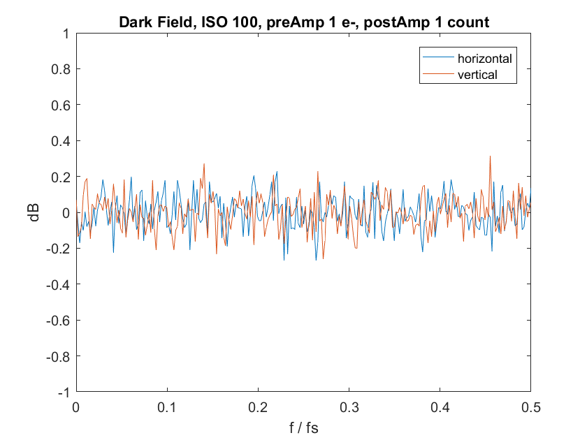
The far left side is zero frequency, sometimes called dc. The far right side is half the sampling frequency of the sensor, and corresponds to the Nyquist frequency. Signals at a higher frequency than the Nyquist frequency will not be properly reconstructed.
You can see that, if you average out the noise, that the plot is flat.
Now let’s set the camera to ISO 3200:
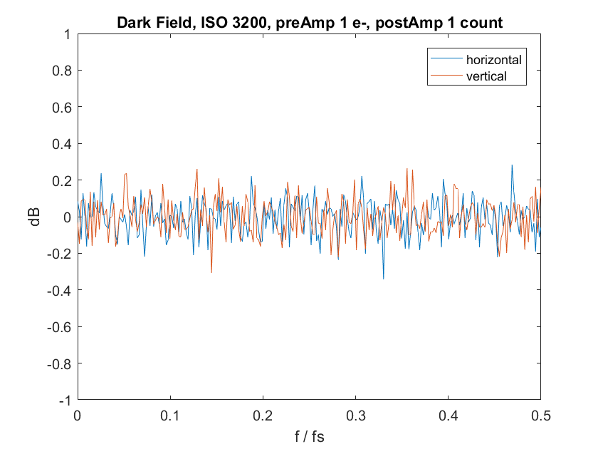
Looks pretty much the same, doesn’t it? But we know there’s more noise at ISO 3200. The reason the graphs look the same is that they are relative to the total noise power. If the total noise power goes up, and the distribution of frequencies in the noise is unchanged, the curve doesn’t change.
Now let’s set the camera back to ISO 100, and expose a uniform image at half scale (one stop down from clipping):
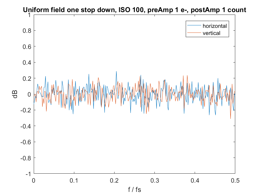
Still the same.
Now I’ll add in the photon noise associated with that half-scale signal:
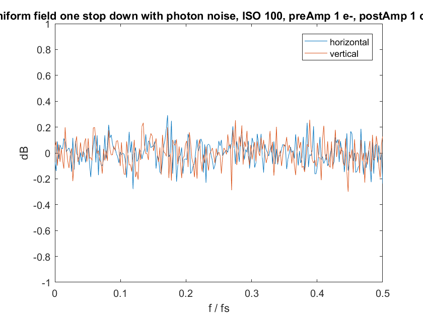
Also still the same. I won’t bore you with another plot, but if I add in Gaussian photon response non-uniformity, that doesn’t make the curves change, either.
What does make them change?
Let’s say that I make every fourth column on the sensor just 0.1% less sensitive than the other columns.
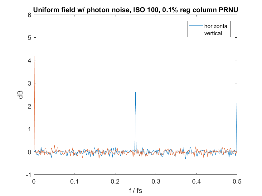
Wow! there is a huge spike in the horizontal direction at one quarter the sampling frequency. Note that I had to change (or, actually, tell the program to change) the scale of the vertical axis or else the spike would have been way off the graph. 0.1% isn’t a lot. So this measurement is very sensitive.
Now let’s say that there is no PRNU, but a 0.1% illumination nonuniformity, in the form of a horizontally-oriented linear gradient with a maximum attenuation of 0.1%:

It’s not as easy to see as the spkie on the graph above it, but there is about a 3.5 decibel rise at dc.
Next up: the effects in the frequency domain of digital signal processing.
Leave a Reply