This is the nineteenth in a series of posts on color reproduction. The series starts here. You don’t have to read the whole thing if you don’t want to. I’ll try to make this post reasonably self-contained. If you get confused, reading the series from the beginning may be useful.
In the previous post in this color reproduction series, I raised the issue of whether the reference colors in a Macbeth chart — and, by extension, in any color accuracy target — should be the patch colors illuminated by the same illuminant as the target, by a standard illuminant such as D50, or by an illuminant which resolves to the white point of the raw processor output color space (D50 for ProPhoto RGB, D65 for Adobe RGB and sRGB).
I have been carrying out an interesting on-line conversation on the subject on DPR. One of the participants in the discussion, quoting Babelcolor, a well known color software web site, said that the adaptation errors add in quadrature with the rest of the profile errors (an incomplete list: capture metameric error, adaptation error, and color profile error). Here’s the quote:
The errors of Table 8 should not be added since they are statistical in nature. The combined effect of multiple processes can be evaluated by calculating the Root-Sum-Squared (RSS) value: Rss_error= [ (error#1)^2+(error#2)^2+ …. ]^(1/2) (20)
[Added later. Originally the person who provided the quote was not able to give me a working link to the paper from whence the above quote came. I now have the link:
http://www.babelcolor.com/index_htm_files/RGB%20Coordinates%20of%20the%20Macbeth%20ColorChecker.pdf
Now that I can read the paper, I see that the errors that Babelcolor considered uncorrelated in the above quote are other errors associated with RGB color space conversion, all of which become immaterially small if the calculations are carried out in double precision floating point and negative values are allowed.
I cannot find any statement by Babelcolor that they expect color errors associated with capture metameric error, profile design and implementation, or raw developer algorithms to be uncorrelated with adaptation errors.]
Since the adaptation errors that I referenced were in general, a fair amount smaller than the rest of the errors, if the two sets of errors added in quadrature (the square root of the sum of the squares) then the adaptation errors that I was finding might not be material.
I though I’d do a test to see how the errors add. I started with a Macbeth chart image from the Sony a7RII, illuminated by a Wescott LED panel pair with the color temperature set to 3200K, developed in Lr 2015 CC with the Camera Standard profile, and output as Adobe RGB.
I also looked at a simulation of the above using a perfect Luther-Ives camera. I have been presenting pretty graphs up to now, but in this post I’m going to stick to boring old tables, the better to show fine differences.
I will be writing Matlab code to compensate for exposure errors and nonlinearities introduced by the raw processor, since I don’t think it presents a fair picture of a raw processor’s color accuracy for normal photography (as opposed to art documentation and reproduction, fabric catalogs, clothing ads, and the like) to penalize the developer for introducing a film-like nonlinear tone curve, which by definition increases CIELab and CIELuv Delta E.
However, I have yet to write that code, so, as an imperfect but workable solution, I’m reporting the color errors as Euclidean distance in CIELab chromaticity space: sqrt(a^2 + b^2). I chose the Lab white point to be the same as that of Adobe RGB. The errors are presented in the same arrangement as the patches on the CC, with the neutral row at the bottom.
Here’s what you get if you illuminate the target with D65 light and sample it with the perfect camera, using the 1931 CIE 2 degree observer:
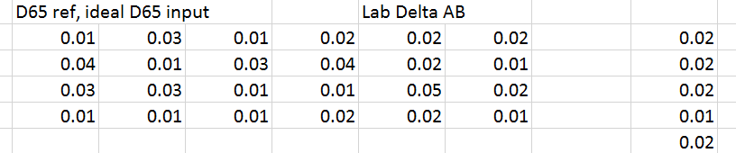
The errors are very small. The right hand column is the average of the rows, and the bottom right number is the average of the errors of all 24 patches.
Now, still using the ideal camera, let’s illuminate the target with Planckian (black body radiated) light at 3200K and keep the reference the patches illuminated by D65 light, and using the Bradford adaptation algorithm to get the target image to the Adobe RGB color space.
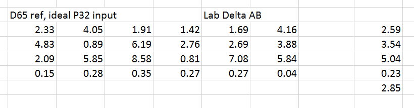
The average error of the gray row is quite low. There are significant errors in the other three rows.
There is one more ideal case to examine. It seems that the X-Rite now reports the color checker colorimetric values as measured under D50 illuminant. So, with the target illuminated with 3200K black body light and converted to Adobe RGB using Bradford adaptation, and the reference values calculated by lighting it with D50 light and and converting to Adobe RGB also using Bradford adaptation, we get the following errors:
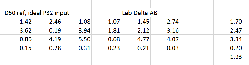
As you’d expect, they are somewhat smaller than the errors where the reference is illuminated with D50 light, since the adaptation from 3200K to D65shares something in common with the adaptation from D50 to D65.
Now we move on to the real camera data. Lr CC 2015 with default settings, except for white balancing to the third gray square from the left, and picking the Camera Standard profile. The reference is the Macbeth chart illuminated by a 3200 degree Kelvin black body radiator. Let’s call this the 3200/3200 case.
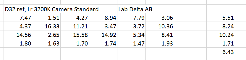
This is not a particularly great profile if accuracy is the goal. There are several colors that are wildly (in this case, I’m defining wildly as more than 10 Delta E) off. The average error is not too bad, though, with the gray row helping a lot.
Now, let’s do the same test, but light the reference with D65 light:
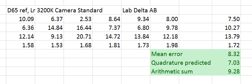
The mean error is almost 2 Delta E worse. If the adaptation error of the ideal camera under similar conditions is added to the 3200/3200 result with the real camera, we get an error that is almost 1 Delta E greater than the measured error. However, if the 3200/3200 error is added in quadrature, the predicted error is well over 1 Delta E too low.
Now let’s light the reference with D50 light:

As you’d expect, the average errors drop. Adding adaptation error in quadrature still is optimistic by more than arithmetic addition is pessimistic.
There are many more accurate profile than this Camera Standard one. As the profiles get better the errors induced by picking the wrong illumination for the reference get even more significant.
Leave a Reply