A week ago I posted some images of Fourier transforms of Siemens Star photographs, and some interesting discussion ensued. Jack Hogan, one of the participants, has written up a guest post showing an interpretation of these plots. I am grateful to Jack for taking the time to do this.
Take it away, Jack:
A few pointers that may help understand what we are looking at on the page of the Fourier transformed images of Siemens star captures.
The image of a Siemens star represents increasing linear spatial frequencies from the rim of the ‘wheel’ to its center. For instance we can see in the image below that near the rim there is one spoke every 18 pixels, while further down there are fewer and fewer pixels between them until… well in the center things become noisy and messed up.
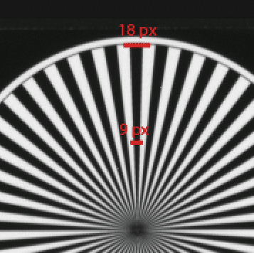
So one period in these images is represented by the linear distance between two spokes.. Frequency is one over the period, so we know that it would be at a minimum at the rim and at a maximum near the center.
The direction in which spatial frequency occurs in the image is going to be perpendicular to each spoke according to its position within it. A Fourier Transform of such an image will measure the relative energy of linear spatial frequencies contained within it. It produces a two dimensional spectrum that looks as follows (loge(magnitudeFT), below right).
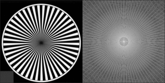
Such graphs are hard to get meaningful quantitative information from because of their scale and because there typically isn’t enough resolution in the z-axis. But we can take a look at its major components.
Say you are sitting in the center of the FT spectrum looking in an easterly direction: the varying intensity along your line of sight represents the relative energy of the various frequencies in that direction (easterly) contained within the image. Each subsequent pixel in the FT image represent 0,1,2,… cycles/set, with 0 in the center in this case.
So for instance, what is that ball near the center? We said that the spokes represented a set of spatial frequencies from maximum near the center to a minimum at the rim. The ball represents the minimum and should have a radius corresponding to a frequency of 284px/18px = 15.75 cycles/set. And sure enough, if we measure its radius it is about that (284 by the way is the width of the Siemens star image, indicating the sample size in that direction). It’s a circle because the spokes are arranged in a circle.
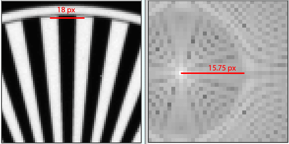
What about those rays emanating out radially in the FT? Aside from giving rise to a frequency interacting with nearby spokes, each spoke is interpreted as a single separate strong line on its own in the original image, giving rise to a line of impulses in the direction of the relative frequency (the direction of the frequency is perpendicular to the direction of the spoke). There are twice as many rays in the FT as there are spokes because the FT does not differentiates between black and white lines.
There was also a question about the apparent replicas of some of the central (baseband) features near the cardinal points and in the corners. The images above were obtained from straightforward processing of the raw data of a Leica Monochrome Typ 216 (L1000865.DNG, if you wish you can download it from DPR’s new studio scene). As you can see its data does not result in such replicas. Yet they are present in the raw data from a D7200 processed exactly the same way, as you can see below (DSC_0532 from the same source) :
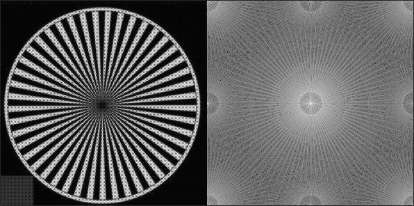
What are they and why are they present in the D7200 and not in the Typ 216? They are aliasing introduced by the Bayer CFA as baseband information is modulated out at cycles/pitch spacing by the color pattern – which the Typ 216, being monochrome, does not have.
The cardinal points here represent the grayscale/luminance Nyquist frequency and should not show aliasing for a pure monochrome image. So they don’t. However same color channel pixels are twice as far in a Bayer sensor, so its Nyquist frequency is half that of its monochrome counterpart, therefore halving its unaliased frequency range. In effect, the introduction of chrominance corrupts the otherwise pristine grayscale channel by bringing aliasing closer in. There is a marvelous series of papers by Eric Dubois and David Alleysson that explain all of this mathematically, see for instance this one.
This ends this quick introduction to the interpretation of macro patterns in 2D FTs of images of a Siemens star. What we are looking at in the FT of your captures are variations on these themes. If the aberrations squeeze the spokes together, we will see higher energy at higher frequencies in the relative position of the FT. If they spread them apart, lower. If they change their direction, that will be reflected in the spectrum as well. Etc. But for quantitative analyses there is as far as I know no substitute for images captured with excellent technique, looking at their spectra one direction and one slice at the time, linearly. I’d be very interested to learn something new and hear from someone who has a different take on this.
Was “see for instance this one” supposed to end in a link?
It was, and it now does. But it appears to be broken. Maybe Jack can help.
Thanks for the catch.
For those interested this is Dubois’ letter
http://www.site.uottawa.ca/research/viva/projects/ibr/publications/EDubois_SPL.pdf
and this is Alleysson’s summary
http://david.alleysson.free.fr/Publications/VCIP08.pdf
There is also a write up on the effect of Bayer CFAs on captured spectrum on ‘Strolls’.
Jack