• site home
  • blog home
  • galleries
  • contact
  • underwater
  • the bleeding edge

the last word

Photography meets digital computer technology. Photography wins -- most of the time.

You are here: Home / The Last Word / Lightroom and Photoshop Exposure controls, part 2

Lightroom and Photoshop Exposure controls, part 2

April 16, 2013 JimK Leave a Comment

[Added after the original post. Eric Chan has informed me that there are two image-processing pipelines in Lightroom: output-referred, and scene-referred. Raw files get the scene-referred pipeline. Integer TIFFs get the output-referred pipeline. Therefore, the TIFF test images are getting a different set of processing than LR applies to raw files.]

In the previous post, I reported that the Exposure controls in Lightroom and Photoshop work differently, and I showed some of the differences in tonality. Today, I’d like to consider color in all three dimensions. The question that I’m trying to resolve is, what are the characteristics of each app’s exposure control when used to develop images that are deliberately underexposed according to the precepts of either Unity Gain ISO, or the Signal-to-Noise (SNR) driven method that I’ve talked about in the last few months.

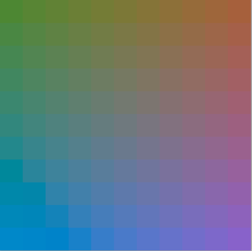
In order to get an appropriate test, I created a test chart consisting of a 11×11 array of squares, with lab values from -50 to +40 in both a* and b*, and a constant L* value of 50 (a middle gray tonality). Here’s the chart, in ProPhoto RGB:

EVtgt

Then I went to my camera simulator program, and created a new camera. It’s in all respects like a Nikon D4, except that it has no noise except for electron and ADC quantizing noise, and a Fovean-like sensor that directly encodes the light into the ProPhoto RGB color space. I know, I know; you could never build a camera like that, especially since two of the PP RGB primaries aren’t physically realizable, but I wanted to minimize color space conversions and errors due to demosaicing.

With my simulated camera, I made five exposures of the target, one at the exposure that replicated the target tonality, and one each at – 1EV, -2 EV, – 3EV, and -4 EV from the first exposure.

I opened each exposure in Lightroom, and used the exposure control to compensate the four underexposed images to about the same RGB values (in the middle of the image) as the normally exposed image. To my surprise, it didn’t take exactly one EV of correction for each EV of underexposure; it took somewhat less.

I exported all the images from Lightroom in ProPhoto RGB, brought them into Photoshop and converted them to CIELab, then brought those images into Matlab and analyzed them.

First, I looked at the chromaticity — only the a* and b* values. Here’s the normally exposed image:

The one-stop underexposed image:

The two-stop underexposed image:

The three-stop underexposed image:

and the four-stop underexposed image:

As you can see, there is a loss of chroma in the blues and magentas.

Then I performed the analogous (but not equivalent) operations in Photoshop, using the Exposure adjustment layer. Like the exposure control in Lightroom, I didn’t have to slide the slider as far to the right as I would have thought. It was much easier to match the levels of the five images, since the Info tool in Photoshop can read out in Lab, something that you can’t do in Lightroom — yet.

Here’s the normal image with no adjustment.

The one-stop underexposed image:

The two-stop underexposed image:

The three-stop underexposed image:

The four-stop underexposed image:

As you can see, Photoshop has exemplary performance when used to boost underexposed images; much better performance than Lightroom. On the other hand, it doesn’t have the lovely soft clipping that you get with the Exposure control in Lightroom.

Next up: three dimensional results.


The Last Word

← Lightroom and Photoshop Exposure controls Lightroom and Photoshop Exposure controls, part 3 →

Leave a Reply Cancel reply

Your email address will not be published. Required fields are marked *

May 2025
S M T W T F S
 123
45678910
11121314151617
18192021222324
25262728293031
« Apr    

Articles

  • About
    • Patents and papers about color
    • Who am I?
  • How to…
    • Backing up photographic images
    • How to change email providers
    • How to shoot slanted edge images for me
  • Lens screening testing
    • Equipment and Software
    • Examples
      • Bad and OK 200-600 at 600
      • Excellent 180-400 zoom
      • Fair 14-30mm zoom
      • Good 100-200 mm MF zoom
      • Good 100-400 zoom
      • Good 100mm lens on P1 P45+
      • Good 120mm MF lens
      • Good 18mm FF lens
      • Good 24-105 mm FF lens
      • Good 24-70 FF zoom
      • Good 35 mm FF lens
      • Good 35-70 MF lens
      • Good 60 mm lens on IQ3-100
      • Good 63 mm MF lens
      • Good 65 mm FF lens
      • Good 85 mm FF lens
      • Good and bad 25mm FF lenses
      • Good zoom at 24 mm
      • Marginal 18mm lens
      • Marginal 35mm FF lens
      • Mildly problematic 55 mm FF lens
      • OK 16-35mm zoom
      • OK 60mm lens on P1 P45+
      • OK Sony 600mm f/4
      • Pretty good 16-35 FF zoom
      • Pretty good 90mm FF lens
      • Problematic 400 mm FF lens
      • Tilted 20 mm f/1.8 FF lens
      • Tilted 30 mm MF lens
      • Tilted 50 mm FF lens
      • Two 15mm FF lenses
    • Found a problem – now what?
    • Goals for this test
    • Minimum target distances
      • MFT
      • APS-C
      • Full frame
      • Small medium format
    • Printable Siemens Star targets
    • Target size on sensor
      • MFT
      • APS-C
      • Full frame
      • Small medium format
    • Test instructions — postproduction
    • Test instructions — reading the images
    • Test instructions – capture
    • Theory of the test
    • What’s wrong with conventional lens screening?
  • Previsualization heresy
  • Privacy Policy
  • Recommended photographic web sites
  • Using in-camera histograms for ETTR
    • Acknowledgments
    • Why ETTR?
    • Normal in-camera histograms
    • Image processing for in-camera histograms
    • Making the in-camera histogram closely represent the raw histogram
    • Shortcuts to UniWB
    • Preparing for monitor-based UniWB
    • A one-step UniWB procedure
    • The math behind the one-step method
    • Iteration using Newton’s Method

Category List

Recent Comments

  • bob lozano on The 16-Bit Fallacy: Why More Isn’t Always Better in Medium Format Cameras
  • JimK on Goldilocks and the three flashes
  • DC Wedding Photographer on Goldilocks and the three flashes
  • Wedding Photographer in DC on The 16-Bit Fallacy: Why More Isn’t Always Better in Medium Format Cameras
  • JimK on Fujifilm GFX 100S II precision
  • Renjie Zhu on Fujifilm GFX 100S II precision
  • JimK on Fuji 20-35/4 landscape field curvature at 23mm vs 23/4 GF
  • Ivo de Man on Fuji 20-35/4 landscape field curvature at 23mm vs 23/4 GF
  • JimK on Fuji 20-35/4 landscape field curvature at 23mm vs 23/4 GF
  • JimK on Fuji 20-35/4 landscape field curvature at 23mm vs 23/4 GF

Archives

Copyright © 2025 · Daily Dish Pro On Genesis Framework · WordPress · Log in

Unless otherwise noted, all images copyright Jim Kasson.