This is the sixteenth in a series of posts on color reproduction. The series starts here.
I’ve spent the last few days coding up a storm so that I can automate the color error calculations involved in analyzing Macbeth color checker charts converted by various cameras, raw developers, and camera profiles.
I needed to test my code, so I came up with a way to simulate a perfect camera, and run the files from that camera through my analysis code. Since the method that I’m using counts on the raw developer’s conversion of the white point of whatever image its presented to the white point of the output RGB file, I needed to perform that white point transformation as well. There are many ways to do this, and two popular algorithms are the old, reliable von Kries method, or the newer Bradford one. Not knowing what method any given raw developer uses, I used both.
I started out with the spectral reflectances of each of the Macbeth patches, and illuminated them with several standard illuminants, D65, D50, E, A, and C. The CIE has tables with the spectral values of these illuminants. I chose Adobe RGB as the output color space. Since the white point of Adobe RGB is D65, the errors with that illuminant should be very low.
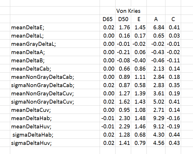
Here are the aggregate measures for von Kries WB adjustment that my simulation spit out.
And here are the errors using Bradford conversion:

The illuminants are across the top, and the aggregate measures run from top to bottom.
Mean Delta E is the average CIELab delta E. It is very low for the two D65 columns, meaning that my code is probably doing its job well. Judged by Lab Delta E, Bradford appears to do a better job of WB correction than the old standard method. Since Delta E can never be negative, errors in one direction don’t cancel out errors in another.
Mean Delta L is the average difference in the CIELab and CIELuv vertical (luminance) channel. Positive Delta L means that the output is brighter than it should be. Negative Delta L means that the output is darker than it should be. Thus Delta L is good for detecting systematic luminance bias.
Mean Gray Delta L is the average difference in the CIELab and CIELuv vertical (luminance) channel for the 6 gray patches. Positive Gray Delta L means that the output is brighter than it should be. Negative Gray Delta L means that the output is darker than it should be. Thus Gray Delta L is good for detecting systematic luminance bias in the gray axis. I will be adding software to correct for exposure variations. Driving the Mean Gray Delta L towards zero will be the job of that code.
Mean Delta A and B are the average differences in the CIELab and CIELuv a and b channels. Positive Delta A or B means that the output is redder or yellower than it should be. Negative Delta A or B means that the output is bluer or more cyan than it should be. These measures are good for detecting systematic color balance bias.
Mean Delta Cab is the average chroma error measured in Lab. A positive number means that the output colors are more saturated than they should be. A negative number means that the output colors are less saturated than they should be.
Mean Non-Gray Delta Cab is the average chroma error measured in Lab for the 18 chromatic patches. Mean Non-Gray Delta Cuv is the average chroma error measured in VIELuv for the 18 chromatic patches. A positive number means that the output colors are more saturated than they should be. A negative number means that the output colors are less saturated than they should be. The sigma metrics track the standard deviation of the 18 samples.
Mean Delta Hab is the average hue angle error measured in Lab, expressed in degrees. The gray patches are excluded from this measure, since their target hue angle is undefined. A positive number means that the output colors have a hue angle higher than they should have. A negative number means that the output colors have a hue angle lower than they should have. Mean Delta Huv is the same measure in CIELuv. The sigma metrics track the standard deviation of the 18 samples.
In case you want to see how these errors appear plotted in CIELab, here’s a look at the Bradford algorithm with Illuminant A.

What’s the dark gray rectangle? Beats me. Some kind of Matlab weirdness, I guess.
When you see the errors from actual raw converters, it will be well to remember that white balance conversion can be a significant source of errors, although in general smaller than those due to the camera, the profile, and the raw developer.
Hi Jim,
Oh, many thanks for that! Wow, You give me an answer of all my try to understandt, why the raw-Converter-software works different, with the same raw-file! When I open a raw-file with Capture One Pro, Lightroom/ACR, DXO, RawTherapee or darktable software (default), you will have a different starting point in color. Because all these software use an other converting algorithm for the whitebalance.
That is annoying and do not help for colorcorrection, even with MacBeth or X-Rite color card!
Maybe you have pointed out the point.