Microcolor and CFA spectra

I found an error (a prime symbol, ‘, omitted) in the code that I used to generate the images in the original post, so I have extensively revised it. My apologies.

In the previous post, I reported on the effect of the selectivity of the color filter array (CFA) spectra on color accuracy in cameras with a Bayer array or something similar. Today I’m going to talk about if and how the CFA selectivity affects another property, with I’m calling microcolor.

There is a small group of people that define microcontrast differently from most of us. The standard definition is contrast at some high spatial frequency — I favor 0.25 cycles per pixel. The people with a different definition say its the differentiation between colors that are very close together. I’m calling that microcolor to avoid confusion here.

This post has been some time in the creating, and I fear that I have invested more time and effort into the research behind it than it’s worth, but it was one of those things where I didn’t realize how hard it was going to be until I had so much time invested into it that I didn’t want to abandon the project.

The idea behind the work that you’re going to see below is to construct pairs of spectra that color-normal humans (I’ll be dropping the “color-normal” part for the rest of the post, but consider it implied) or the 1931 CIE 2-degree Standard Observer would say are close together, present those spectra to simulated cameras with different CFA response spectra, and measure the distance between color pairs as seen by the camera. This test does not measure color accuracy; we already looked at that (and noise) for the Macbeth CC24 patches, and may in the future look at that for small (and, what the hey, large) deviations from them. But in this post, I’m concerned with how different are pairs of colors as seen by the camera as compared to how different are pairs of colors as seen by a human. A camera with low microcolor would see smaller color differences than a human. A camera with high microcolor would see larger color differences than a human.

Here’s my methodology:

• Write a camera simulator that takes as input the Macbeth CC24 spectra, a set of CFA/sensor response spectra, and a standard light source (I used D50).
• Program the simulator to create optimal compromise matrices for going from raw values to CIE XYZ.
• Create pairs of spectra that resolve to colors a fixed distance apart. For this post, I’m using CIELab DeltaE 2000 as the distance metric.
• Measure the distances, in CIELab DeltaE 2000, between these pairs after the camera’s raw files are converted to CIE colors using the optimal compromise matrices.
• Compare the two distances.

I thought hard about how to create the pairs of spectra. I finally decided to use the spectra of the Macbeth CC24 as basis functions. I took all 18 chromatic patches on the Macbeth CC24 chart (excluding the neutral bottom row of 6 patches), and mixed each one with the other 23 patches to create pairs with predetermined CIELab DeltaE 2000 distances. Thus there were 18 sets of pairs, one with each of the patches as the base, and 23 pairs in each set.

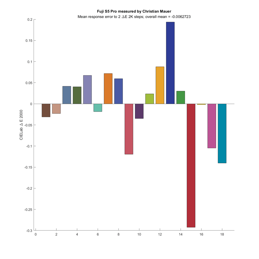
Here are the results for a set of CFA response spectra that match the CIE 1931 XYZ spectra:

 

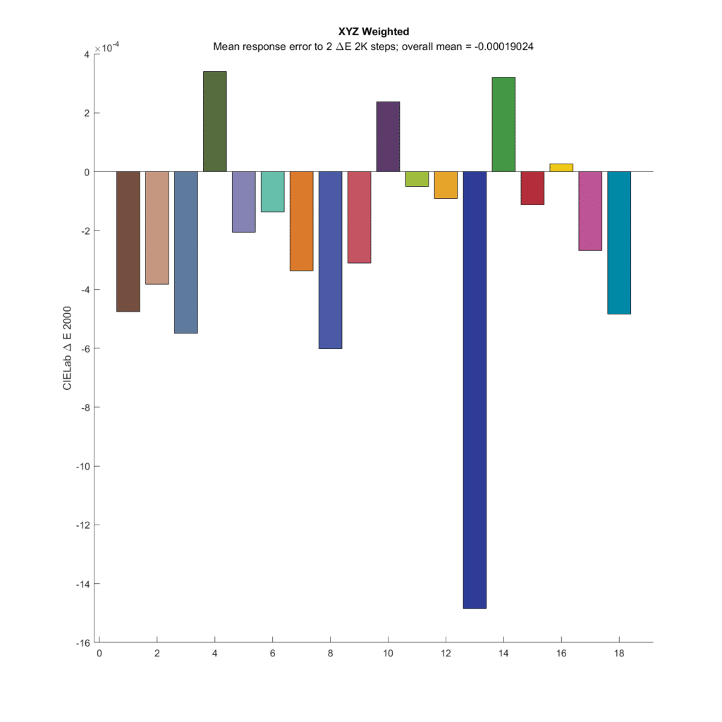
The original pairs were all 2 DeltaE 2000 apart. What’s plotted for each chromatic patch is the average difference between the 23 pairs with that patch as the base, less the 2 DeltaE 2000 distance of the original pairs.  If the camera were perfect, All the bars would be zero. I’ve colored each of the bars with the color of the base patch in each set. The first thing to notice is how small the errors are. The vertical axis of the graph goes from -0.0016 to 0.0004 Delta E 2000. All the errors are very small. This is in spite of the fact that the compromise matrix created by the optimization program wasn’t quite the right one.

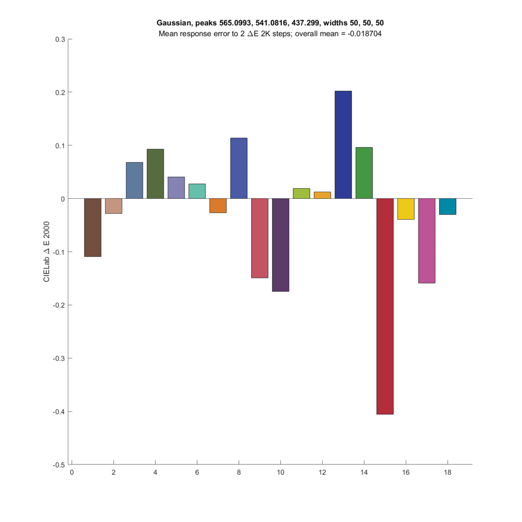
Next up is the optimal Gaussian CFA set from the preceding post.

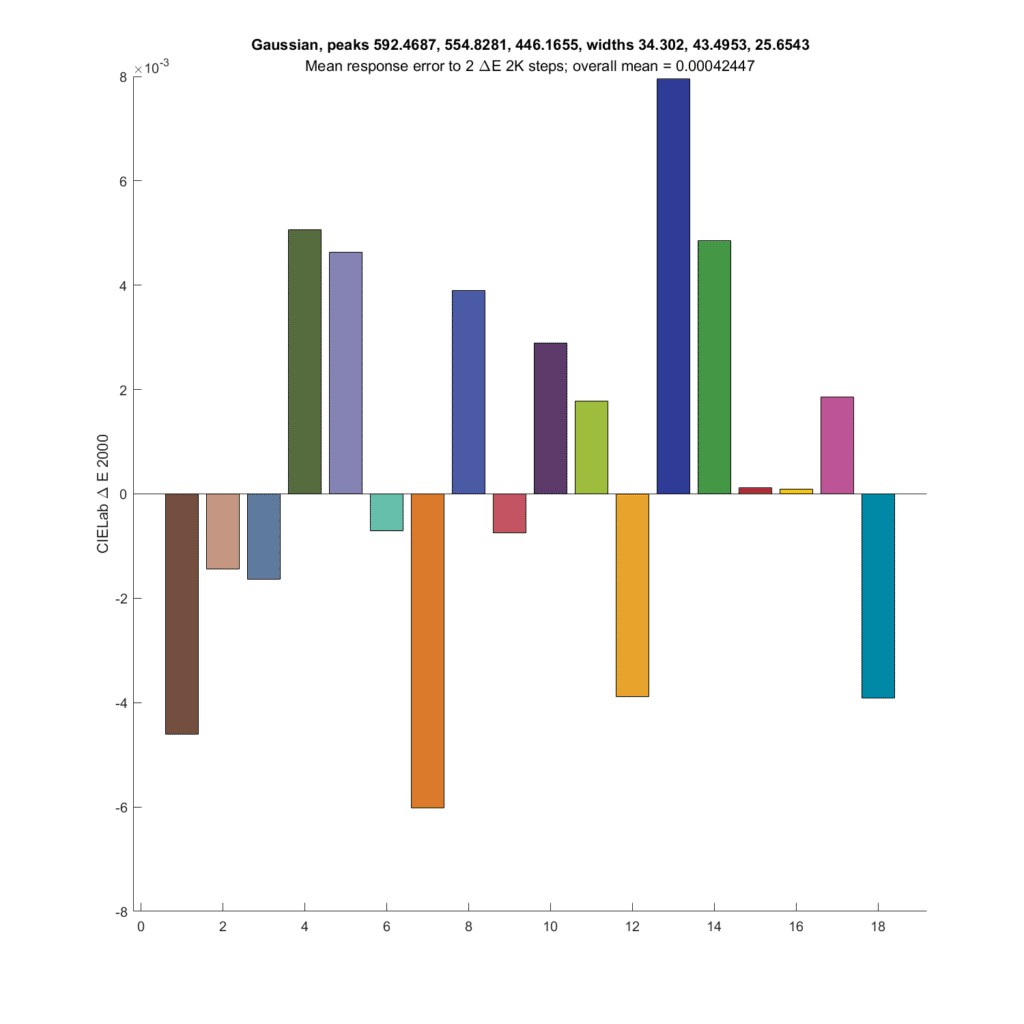
The results are not as good as the CIE XYZ CFA set. Both the XYZ set and the Gaussian set above have about the same SMI; 99.3 for the Gaussian and 99.7 for the XYZ.

The people I was talking about at the top of this post say that narrower CFA spectra produce higher microcontrast microcolor. Let’s make the spectra narrower, with standard deviations of 20 nanometers. The peak frequencies are optimal for those standard deviations.

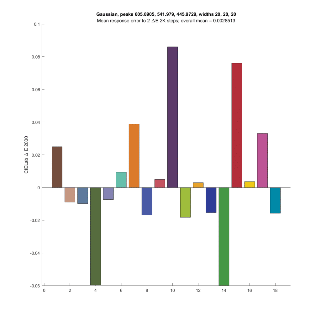
The errors are quite a bit greater, but still low at worst less than a twentieth of the actual shifts in DeltaE 2000.

 

Now I’ll make the standard deviation (sigma) even narrower, with optimal peak wavelengths:

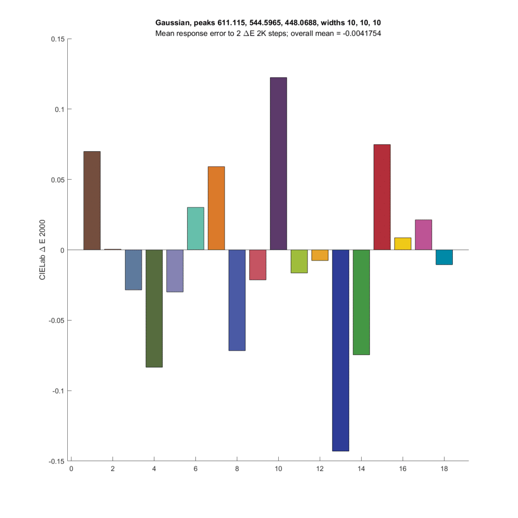
The average microcolor metric  is now slightly negative. The errors are in general larger.

Does making the sigma really wide (with optima peak wavelengths) make the microcolor metric go negative?

On average, it does not do so significantly, although there are some very large swings, but they tend to cancel each other out.

Let’s look at a camera that did quite well in the past simulations, the Arriflex D21:

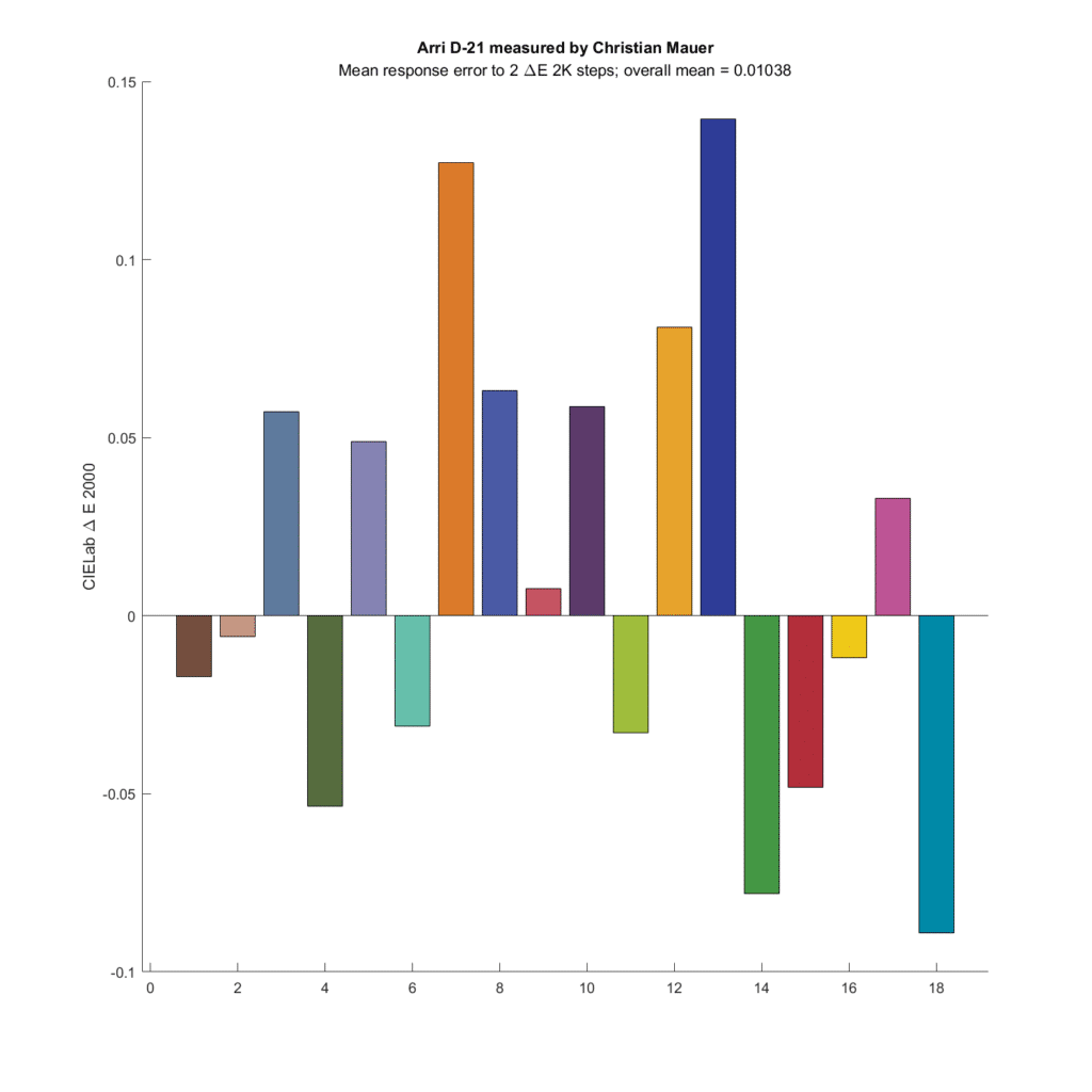
The average color error is very slightly greater than zero.

How about a couple of old CCD cameras?

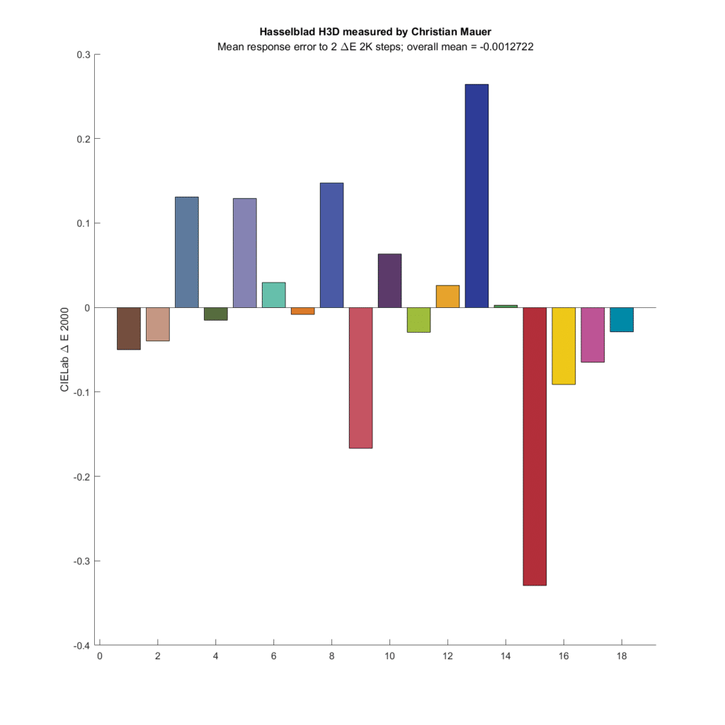
The Hasselblad has a quite a bit of microcolor variation, and on average, shows a bit tiny bit less difference than the simulated eye sees.

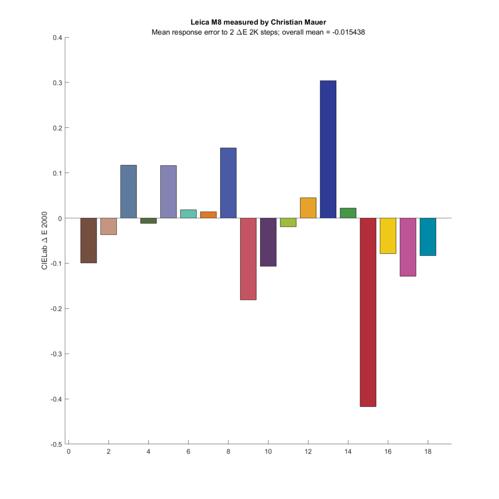
So does the Leica M8, although most of the difference comes from a small number of patches.

Some more cameras:

My conclusions are:

• Microcolor is a real thing: for some base colors, cameras/raw developers can show larger or smaller changes in captured color differences than observed by  the eye.
• The effect is small, even with the color patches most affected
• Average microcolor changes across all colors are tiny.
• I see no evidence that narrower CFA spectra means more microcolor.
• There is wide variation in microcolor as the base patch values change.
• The two CFA spectra that produce the most accurate color produce the microcolor that most agrees with what the eye sees
• The optimum Gaussian spectra produce slightly more microcolor errors than an ideal spectra set.