As many of you know, I’ve been doing slit scans of plants, and I’ve been struggling with image artifacts due to subject motion. In the past few days I’ve been working on a Matlab program to deal with the artifacts and at the same time assemble several images into a complete, visually seamless composite.
In this post, I’ll walk through what the program does, and how it does it. The reason for posting this level of detail is not mainly to help out the photographers who are doing the same kind on photography — I figure that they’re thin on the ground — but to give those of you with some programming skills the kinds of things that you could do that might help your own photography by allowing you to do things that you can’t do in Photoshop and automate things that you have to do manually in Ps.
The files that form the basis for the final image are 14 in number, each one a 58176×6000 pixel TIFF produced by a Betterlight SUper 6K scanning back. Each file represents about 45 minutes total exposure. The program optionally performs median filtering on the images with a kernel that’s 128 pixels in the time direction and 1 pixel in the other one, reduces the number of pixels in the time direction by a factor of 16 using an algorithm calculated to average out noise, assembles all the images into one, then performs more median filtering. It writes out all the individual files and a series of composite ones with varying amounts of median filtering.
The first part of the program is just housekeeping, setting up file names and a few constants:
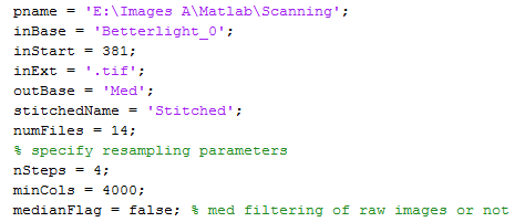
Median filtering is a computationally-intensive operation for large extents, and Matlab’s implementation does no parallelization, at least if you don’t have the parallel processing toolkit. Using 128×1 extents on the original files took a long time and, although it removed most of the artifacts, it didn’t get them all. So I was pleased to find that using a 8×1 extent on the files that had been compressed by a factor of 16 in the time dimension produced substantially the same results. I left the median filtering in the program, but made it optional, and turned that option off.
The way I compress the files in the time dimension is through repeated applications of bilinear interpolation, reducing the size of teh file by a factor of two at each step. The program next sets up a array of image sizes:
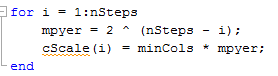
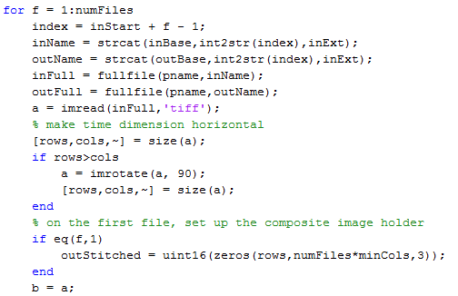
Then I read in the files, rotate them if necessary (Betterlight and Matlab don’t always see eye to eye on orientation), and (the first time around) set up the image container that will receive the composite image.
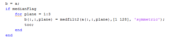
Then I do the median filtering if it’s desired:
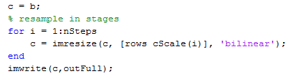
Then I do the successive resamplings and write out the files:
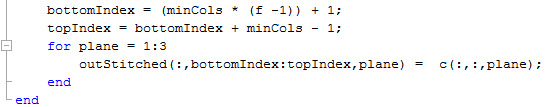
Finally (for this for loop, anyway), I put the squeezed files into the composite container:
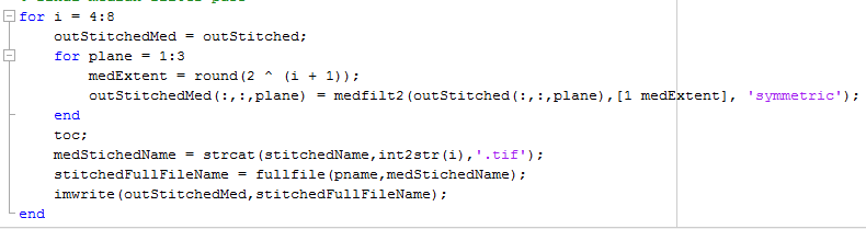
All that’s left is to do various amounts of median filtering and write out the filtered composite files:
There are short-duration disturbances due to wind, and longer ones that are caused by insects crawling around on the leaves of the plant. I thought at first that I’d have to pick between different extents of median filtering depending on what was going on minute to minute. However, I was pleasantly surprised to find that there was no perceptible degradation to the image sharpness even when using extents of 512 (!) pixels.
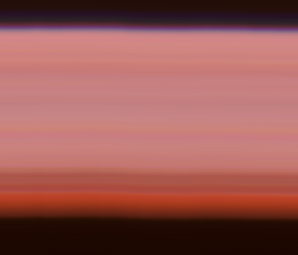
Here’s a insect-driven (slow) artifact with an extent of 32×1:
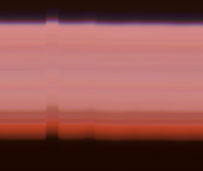
It’s softened, but still ugly.
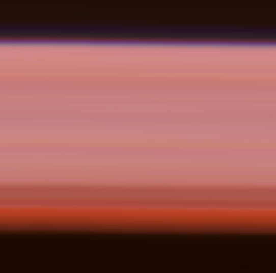
With an extent of 64×1, it looks like this:
Almost all gone.
Doubling the extent again to 128, we get this:
A hair better.
It looks like this operation is not going to require any hand tweaking, at least for the succulent pictures.
Success here has emboldened me to go back to subjects whose motion had stymied me in the past, like trees with blowing branches. More to come.
Leave a Reply