Yesterday I went back and looked at some of the simulation results, and grew suspicious that there were problems with the way the simulated camera was sampling the simulated target. As I dug deeper, I started to question some of my original assumptions, and started experimenting with changes. What I ended up with is close to, but not identical to, where I started. I will modify the posts of the last couple of days to reflect the small changes, but today I’d like to report on what I changed and why.
Warning, this will get detailed and geeky.
First off, let me explain how the simulator works. I start off with a RGB target image of about 12000×8000 pixels. I want to end up with a simulated sampled image that’s much smaller. How much smaller? Good question. Stay tuned.
Most of the simulation operates at the resolution of the target. I know the pixel pitch of the sampled image, and I can calculate the ratio of the size of the target to the size of the sampled image. That allows me to compute kernels to apply to the target in terms of the dimensions of the simulated sensor. The first thing that happens is that I construct a kernel to simulate diffraction, and apply it to the target. There are actually three kernels, one for each color plane, and they are computed assuming red light at 650 nm, green light at 550nm and blue light at 450 nm. Then I apply kernels to simulate lens defects. Then motion blur, if any. Then AA filters, if any, Then the sampling of the sensor – this is where the fill factor comes in. Then I do a point sample of the target image to the resolution of the sensor, assigning color planes to sensels with the RGGB Bayer CFA. Next, I add photon noise if desired. Photon noise is not a useful addition for slanted edge spatial frequency response analysis, since the algorithm averages out noise. Then I digitize at the desired precision; I’ve been using 14 bits for the MTF studies.
Now I have a simulated raw file. I “develop” it with bilinear interpolation demosaicing, and feed the resultant RGB image to Dr. Burns’ sfrmat3 function for the MTF analysis, and either save the results, or compute indirect measures from the MTF curves, like MTF50 and MTF 30 and save those measures.
What could go wrong?
The first thing that made me nervous was the amount of energy above the Nyquist frequency with diffraction-limited lenses at wide apertures. The second was instability in the MTF30 and MTF50 results when I ran series with close spacing between the f-stop or pixel-pitch values. With factors of 1.05 between the data points, I saw saw-tooth ripples in the results. Both of those things made me think that I wasn’t sampling the target right.
Was the target resolution sufficiently greater than the sensor resolution? I recoded the sim so that the ratio of the two resolutions was an explicit input, then I ran series with diffraction-limited lenses and perfect AA-less sensors – the toughest cases – at ratios of 8, 16, 32, and 64. 32 and 64 were substantially identical, but the other two were different. That told me that I needed target resolution of at least 32 times the simulated sensor resolution. That was a surprise.
The next thing to look at was sampling jitter. Before, the ratio between the target and the sensor could be anything. But I could only sample at integer target pixel indices. I thought about coming up with a way to interpolate between target pixels, but in the end, I took a simpler approach: crop the target so that it has dimensions that are integer multiples of the sensor resolution and the target to sensor ratio, which I constrained to an integer power of two. Thus the distance, measured in target pixels, between the sensor samples is fixed. Once I’d eliminated the sampling jitter, the MTF50 instability went away.
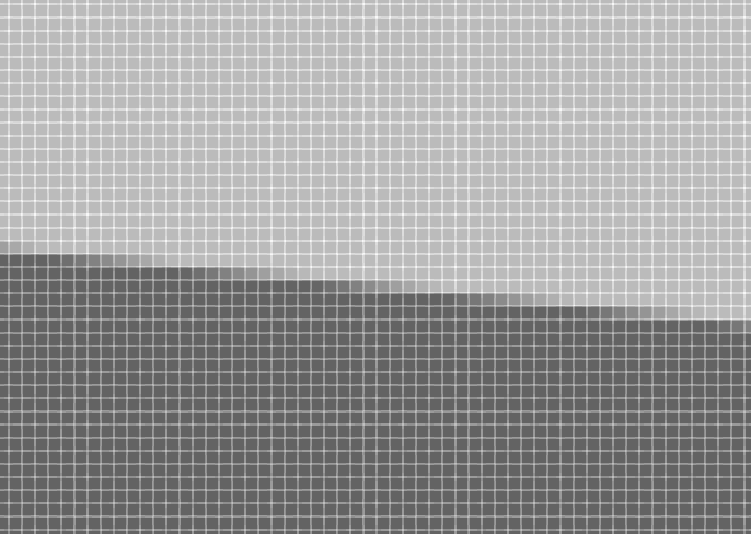
By the way, the target is already aliased. Here’s a close-up:
I still had a lot of aliasing. Was it real? I took a look at some of the simulated demosaiced images. Here’s one for an f/2.8 diffraction-limited lens on a sensor with 100% fill factor:
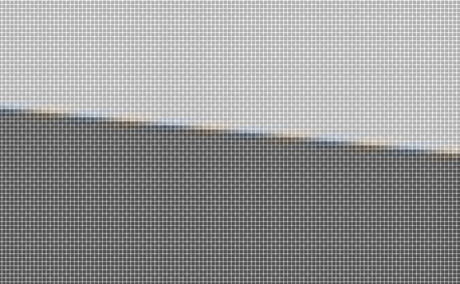
Aliasing? I’ll say! Want to see it at 1% fill factor?
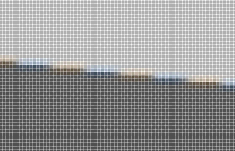
Now that’s just silly, but I don’t think I can blame the SFR analysis for the aliasing.
So, at the end of all this technological navel gazing, I’m pretty much back where I started. I’ve tweaked the model to be more accurate, but my early results were darned close. At least my level of confidence has improved.
Why don’t other people see this much high-frequency stuff in their simulations? The ones I’m most familiar with are looking at raw channels, not demosaiced images, and that makes all the difference. Why don’t I look at raw channels, too? That’s not what I’m interested in; I want to know about aliasing in demosaiced images. I can’t print raw ones.
Jim, could what you call color aliasing above be simply chromatic aberrations created by the edge not being perfectly aligned in each of the ‘three’ raw channels?
CA will result in a degraded MTF50 reading but most raw converters are pretty adept at getting rid of it therefore recovering some of that lost resolution.
Jack, the simulated lens has no chromatic aberration. The sensels are perfectly aligned, too. Of course, they’re looking at different parts of the image because of the Bayer array, which is the source of the false color. If they we all looking at the same part of the image, as in a Foveon sensor, there wouldn’t be the same kind of false color.
Jim
Hi Jim,
I am glad you also saw that we need an unexpectedly high oversampling factor to produce accurate simulated images.
My approach to sampling is render each pixel in the (low res) simulated pixel by generating a very large number of sampling points (roughly corresponding to the pixels in your high-res image, but not aligned to any grid) using an importance-sampling strategy.
I arrived at this particular solution exactly because of the ridiculously high oversampling I saw with the grid-based approach — I went up all the way to 256x oversampling, and still saw some improvement. Later I decided that the grid-based sampling is inefficient — this appears to be mostly because the diffraction MTFs are infinite, and any grid-based sampling (with diffraction simulated as a FIR filter) truncates the MTF in an undesirable way. I particularly noticed that the diffraction MTF would end up with too much power (contrast in the MTF plot) near the very low frequencies; this is a direct result of using a finite-size FIR filter.
The importance sampling approach allows me to take the same number of samples (corresponding to FIR filter taps), but to distribute them to balance the low and high frequency accuracy of the diffraction simulations. I have no real justification for this, other than that it allowed me to generate simulated images that produced measured MTF curves that agreed well with the expected analytical MTF functions. I suspect these differences are well below what is clearly visible in a simulated image anyway.
Just as a side note, the rather pronounced demosaicing false colour you are seeing can be suppressed by the more sophisticated demosaicing algorithms. Of course, they just make a different set of assumptions, and therefore mess up some other type of image feature. I can recommend libraw — they have a good selection of demosaicing methods to choose from.