• site home
  • blog home
  • galleries
  • contact
  • underwater
  • the bleeding edge

the last word

Photography meets digital computer technology. Photography wins -- most of the time.

You are here: Home / The Last Word / Noise reduction and downsampling

Noise reduction and downsampling

September 17, 2014 JimK 5 Comments

[Note. The bilinear and bicubic interpolation algorithms referred to in this article are the Matlab implementations. They are different from the Photoshop algorithms of the same or similar names. The Photoshop versions are reported on a few posts further on. Therefore, this post is primarily of academic interest.]

It is axiomatic in photography that photon noise decreases upon downsampling in direct proportion to the magnification ratio — the width (or height) of the output image over that of the input image.

Downsampling by a factor of two should cut the noise in half. That’s what would happen if you averaged four input image pixels for every pixel in the output.

This reasoning is one of the bases for photographic equivalence. It’s at the root of the way that DxOMark compares cameras of unequal pixel count. It’s accepted without  much thought. I qualify my statement, because there are some who don’t buy the notion.

It’s clear to me that binning pixels — averaging the values of adjacent captured pixels before or after conversion to digital form — will reduce photon noise as stated above, although the two operations have different effects on read noise. What’s not clear is how good the standard ways that photographers use to reduce image size are at reducing noise.

I set out to do some testing. I wrote a Matlab program that I’ll be posting later that created a 4000×4000 monochromatic floating point image, and filled it with Gaussian noise with a mean of 0.5 and standard deviation of 0.1. I then downsampled it using various common algorithms: bilinear interpolation, bicubic interpolation, Lanczos 2 and Lanczos 3. at 200 different output image sizes, ranging from the same size as the input image to less that 1/8 that size in each dimension.

Then I measured the standard deviation of the result. That’s the same as the rms value of the noise. If downsampling operates on noise the way that photographic equivalence says it does, then we should get curves that look like this:

ideal rms noise

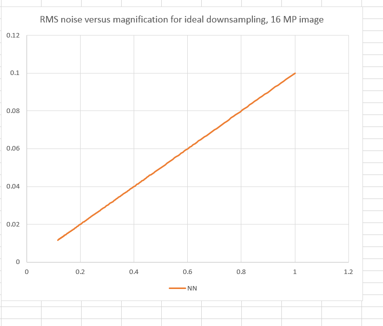
But that’s not what happens. Instead, our curves look like this:

rms no aa

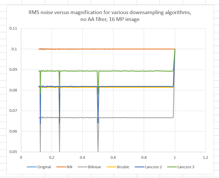
Whoa! Except for some “magic magnifications” — 1/2,  1/4, and 1/8 — the noise reductions are all the same for each algorithm. Bilinear interpolation is the best; it hits the ideal number at a magnification of 1/2, and the sharper downsampling algorithms are all worse. None of the algorithms do to the noise what we’d like them to do.

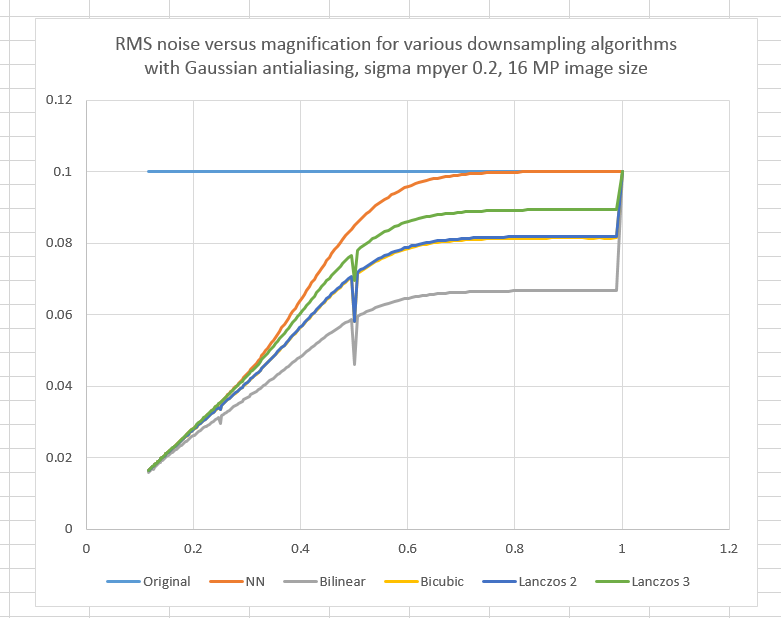
Bart van der Wolf is a smart guy who has looked extensively at resizing algorithms.  One of the things he recommends is subjecting the image to be downsampled to an Gaussian anti-aliasing (AA) filter whose sigma in pixels is 0.2 or 0.3 over the magnification.

Here’s what you get with a AA sigma of 0.2/magnification:

rmsp2gaussian

And here are the curves with sigma equal to 0.3 / magnification:

rmsp3gaussian

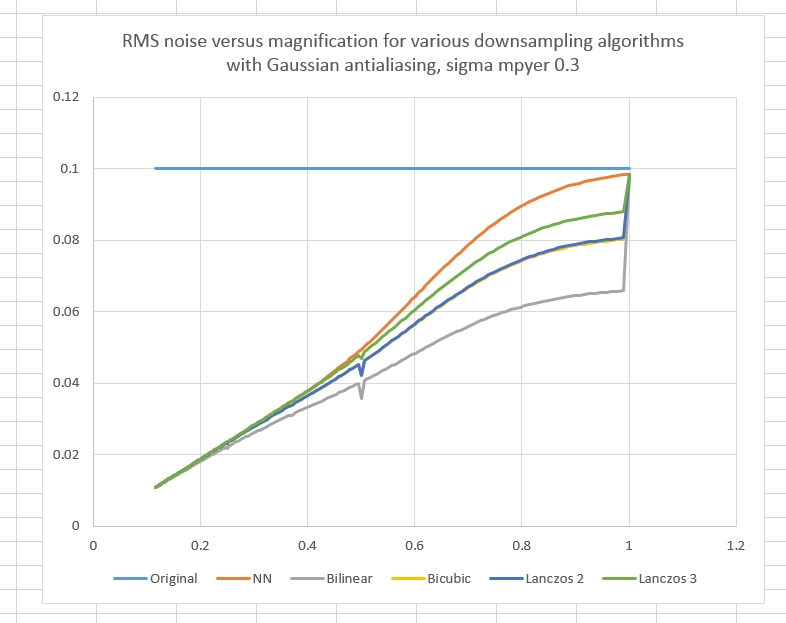
Well that’s better. With 0.3 / magnification, by the time we get to 1/4 size, we’re pretty much on the ideal curve.

But what does the AA filter do to image detail? Are the downsampled noise images still Gaussian? What would happen if we downsampled in a gamma-corrected color space? What about the demosaicing process? What do these algorithms have to do with the ones built into Photoshop and Lightroom?

Stay tuned.

The Last Word

← Museum of Monterey opening Noise reduction and downsampling with a gamma of 2.2 →

Comments

  1. Federico says

    July 2, 2020 at 6:26 pm

    It’s unfortunate that Eolf’s site is gone and with it all that was published.

    Reply
    • JimK says

      July 3, 2020 at 7:28 am

      That’s true. I have removed the now-broken link. Thanks.

      Reply
      • Ken says

        January 3, 2021 at 5:34 am

        The previous broken link appears to have already been to the Wayback machine but just the wrong date to capture Bart’s page before it disappeared.

        This Wayback link is referenced to about when the blog post was originally written and Bart’s page was still active and archived then:

        http://web.archive.org/web/20141027051036/http://bvdwolf.home.xs4all.nl/main/foto/down_sample/down_sample.htm

        Reply
  2. Joost says

    April 6, 2021 at 5:25 am

    Nice article, can you share the 4k image please?

    Reply
    • JimK says

      April 6, 2021 at 6:23 am

      I no longer have the originals. It’s been seven years.

      Reply

Leave a Reply Cancel reply

Your email address will not be published. Required fields are marked *

May 2025
S M T W T F S
 123
45678910
11121314151617
18192021222324
25262728293031
« Apr    

Articles

  • About
    • Patents and papers about color
    • Who am I?
  • How to…
    • Backing up photographic images
    • How to change email providers
    • How to shoot slanted edge images for me
  • Lens screening testing
    • Equipment and Software
    • Examples
      • Bad and OK 200-600 at 600
      • Excellent 180-400 zoom
      • Fair 14-30mm zoom
      • Good 100-200 mm MF zoom
      • Good 100-400 zoom
      • Good 100mm lens on P1 P45+
      • Good 120mm MF lens
      • Good 18mm FF lens
      • Good 24-105 mm FF lens
      • Good 24-70 FF zoom
      • Good 35 mm FF lens
      • Good 35-70 MF lens
      • Good 60 mm lens on IQ3-100
      • Good 63 mm MF lens
      • Good 65 mm FF lens
      • Good 85 mm FF lens
      • Good and bad 25mm FF lenses
      • Good zoom at 24 mm
      • Marginal 18mm lens
      • Marginal 35mm FF lens
      • Mildly problematic 55 mm FF lens
      • OK 16-35mm zoom
      • OK 60mm lens on P1 P45+
      • OK Sony 600mm f/4
      • Pretty good 16-35 FF zoom
      • Pretty good 90mm FF lens
      • Problematic 400 mm FF lens
      • Tilted 20 mm f/1.8 FF lens
      • Tilted 30 mm MF lens
      • Tilted 50 mm FF lens
      • Two 15mm FF lenses
    • Found a problem – now what?
    • Goals for this test
    • Minimum target distances
      • MFT
      • APS-C
      • Full frame
      • Small medium format
    • Printable Siemens Star targets
    • Target size on sensor
      • MFT
      • APS-C
      • Full frame
      • Small medium format
    • Test instructions — postproduction
    • Test instructions — reading the images
    • Test instructions – capture
    • Theory of the test
    • What’s wrong with conventional lens screening?
  • Previsualization heresy
  • Privacy Policy
  • Recommended photographic web sites
  • Using in-camera histograms for ETTR
    • Acknowledgments
    • Why ETTR?
    • Normal in-camera histograms
    • Image processing for in-camera histograms
    • Making the in-camera histogram closely represent the raw histogram
    • Shortcuts to UniWB
    • Preparing for monitor-based UniWB
    • A one-step UniWB procedure
    • The math behind the one-step method
    • Iteration using Newton’s Method

Category List

Recent Comments

  • bob lozano on The 16-Bit Fallacy: Why More Isn’t Always Better in Medium Format Cameras
  • JimK on Goldilocks and the three flashes
  • DC Wedding Photographer on Goldilocks and the three flashes
  • Wedding Photographer in DC on The 16-Bit Fallacy: Why More Isn’t Always Better in Medium Format Cameras
  • JimK on Fujifilm GFX 100S II precision
  • Renjie Zhu on Fujifilm GFX 100S II precision
  • JimK on Fuji 20-35/4 landscape field curvature at 23mm vs 23/4 GF
  • Ivo de Man on Fuji 20-35/4 landscape field curvature at 23mm vs 23/4 GF
  • JimK on Fuji 20-35/4 landscape field curvature at 23mm vs 23/4 GF
  • JimK on Fuji 20-35/4 landscape field curvature at 23mm vs 23/4 GF

Archives

Copyright © 2025 · Daily Dish Pro On Genesis Framework · WordPress · Log in

Unless otherwise noted, all images copyright Jim Kasson.