One-dimensional sharpening

In the last couple of posts, I talked about how to smooth slit-scan photographs in the time direction. For the time being, I consider that a solved problem, at least for the succulents images.

These images require a lot of sharpening, because

• the subject has a lot of low-contrast areas
• there’s a lot of diffraction, because I’m using an aperture of f/45 on my 120mm f/5.6 Micro-Nikkor ED
• even with that narrow f-stop, there are still parts of the image that are out of focus

I’ve been using Topaz Detail 3 for sharpening. It’s a very good program, allowing simultaneous sharpening at three different levels of detail, and having some “secret sauce” that all but eliminates halos and blown highlights. Like all sharpening programs that I’d used before this week, it sharpens in two dimensions.

However, I don’t want to sharpen in the time dimension, just the space one. Sharpening in the time dimension will provide no visual benefits — I’ve already smoothed the heck out of the image in that dimension — and could possible add noise and undo some of my smoothing.

I decided to write a Matlab program to perform a variant of  unsharp masking in just the space direction.

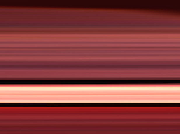
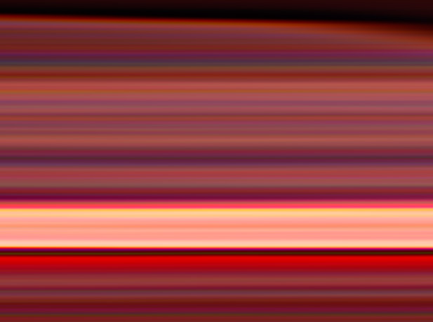
To review what one of the succulent images looks like after stitching and time-direction smoothing cast your eyes upon this small version of a 56000×6000 pixel image:

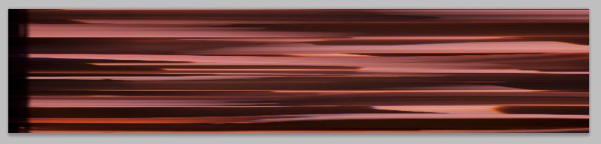
The horizontal direction is time; the image will be rotated 90 degrees late in the editing process. The vertical direction is space, and is actually a horizontal line when the exposure is made.

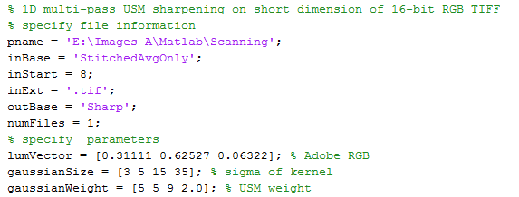
Here’s the program I’m using to do sharpening in just the vertical direction, using a modification of the technique described in this patent.

First, I set up the file names, specify the coefficients to get luminance from Adobe RGB, and specify the standard deviations (aka sigmas) and weights of as many unsharp masking kernels as I’d like applied to the input images. There are four sets of sigmas and weights in this snippet:

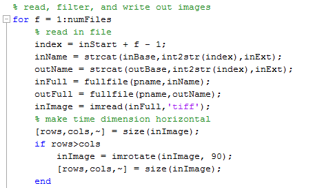
Then I read in a file and rotate the image if necessary so that the space direction is up and down:

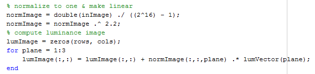
I convert the image from 16-bit unsigned integer representation to 64-bit floating point and remove the gamma correction, then compute a luminance image from that:

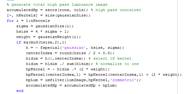
I create a variable, accumulatedHp, to store the results of all the (in this case, four) high-pass filter operations, create a two-dimensional Gaussian convolution kernel using a built-in Matlab function called fspecial, take a one-dimensional vertical slice out of it, normalize that to one, apply the specified weight, and perform the high-pass filtering on the luminance image and store the result in a variable called hpLum, and accumulate the results of all the high-pass operations in accumulateHp:

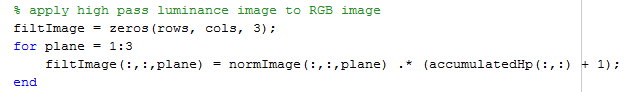
The I add one to all elements of the high-pass image to get a usm-sharpened luminance plane, and multiply that, pixel by pixel by each plane of the input image to get a sharpened version:

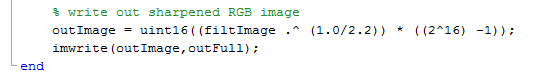
Finally, i convert the sharpened image into gamma-corrected 16-bit unsigned integer representation and write it out to the disk:

How does it work?

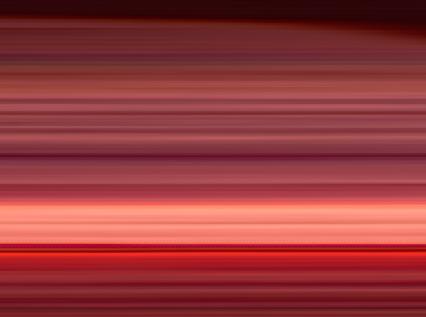
Pretty well. Here’s a section of the original image at 100%:

And here it is one-dimensionally sharpened with sigmas 3, 5, 15 and 15 pixels, and weights of 5, 5, 5, and 2:

If we up the weight of the 15-pixel high-pass operation to 9, we get this:

For comparison, here’s what results from a normal two-dimension unsharp masking operation in Photoshop, with weight of 300% and radius of 15 pixels:

Finally, here’s what Topaz Detail 3 does, with small strength, small boost, medium strength and medium boost all set to  0.55, large strength set to .3 and large boost to 0:

One thing that Topaz Detail does really well is keep the highlights from blowing out and the blacks from clipping. I’m going to have to look at that next unless I decide to bail and just do light one-dimensional sharpening in Matlab and the rest in Topaz Detail.