Sensor photon transfer analysis: PRNU

There are two groups of exposures that need to be made to characterize the photon transfer characteristics of a sensor. Both are flat-field images. If you want to use a white or gray card, illuminate it evenly, defocus the lens, use a fairly long focal length (135mm is my favorite), and crop to the central 400×400 pixel part of the frame. What I’ve found works even better is to put an ExpoDisc on the lens, and aim it straight at the light source. Artificial lighting works best, because it is more repeatable than natural lighting. I use Fotodiox LED floods or Paul Buff Einstein strobes. Both allow the illumination to be varied in intensity, which is sometimes useful.

The first group of exposures is aimed at finding the photon response nonuniformity (PRNU). It is a long series of images — I usually use 256 — made of a flat field at base ISO and an exposure that is close to, but less than, that which would result in clipping. Averaging many of these images averages out the photon noise, which changes with each frame, and leaves the PRNU, which doesn’t. Taking the standard deviation as each new image is averaged in gives an indication of how fast the operation is converging. There is a problem with this approach. It is virtually impossible to get a target that has as little illumination nonuniformity as the camera’s PRNU. The only way that Jack and I have found to deal with this is to apply some sort of high-pass filtering to the averaged image, so that the low-spatial-frequency variations caused by the lighting nonuniformity are suppressed. Unfortunately, if there’s any low spatial frequency PRNU, that will also be suppressed.

The high pass kernel size and the size of the cropped image (sometimes called the region of interest (ROI) extent) will both affect the calculated value for PRNU.

Here are some examples, using the Nikon D4 as the test camera. Values for all four raw channels are plotted after each new image is added in, so you can see how fast convergence occurs. First, with a 400×400 pixel ROI and a 99×99 pixel high pass kernel:

And then with the same ROI and a 7×7 high pass kernel, which will reject more low-frequency information:

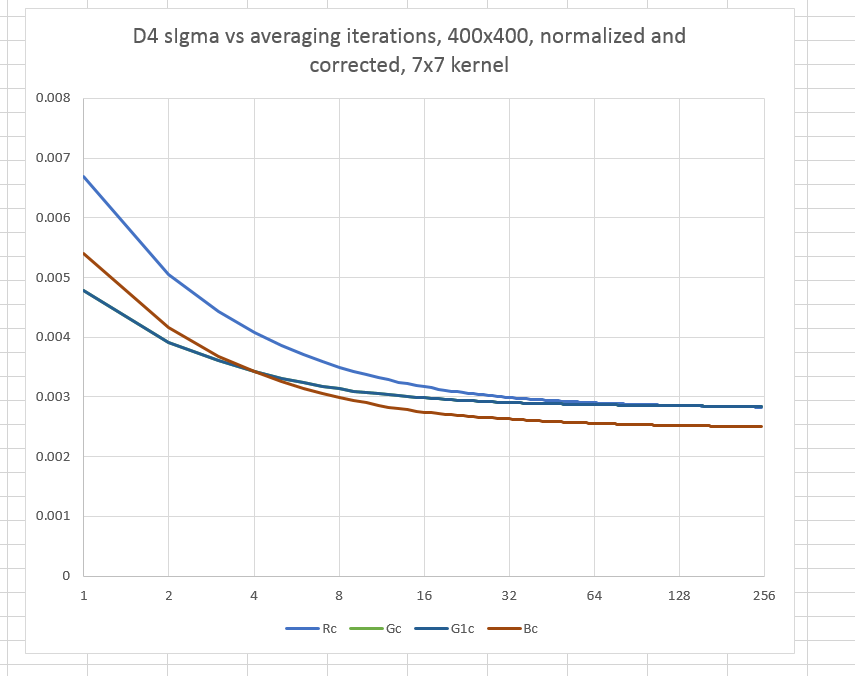
You can see that the kernel size makes the difference between the PRNU being about 0.4% and 0.3% in this case. You can also see that once you get up to 64 images being averaged, very little changes as you add more.

Here’s an ugly truth about measuring PRNU. Dust looks like PRNU. Unless the sensor is pristine — and I’ve never seen one perfectly clean — the PRNU is going to look worse than it actually is.

One way to get a sense of what’s going on with the PRNU is to look at the spectra of the averaged image. Here’s a look at the D4 image before it get’s high-pass filtered:

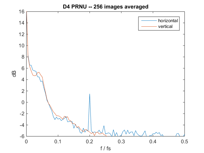
The hump on the left is mostly due to lighting nonuniformity.  I’m not sure what the shelf just above 1/10 the sampling frequency is. The spike in the horizontal frequency spectrum at 1/5 the sampling frequency is probably related to sensor design.

We can get a better idea by looking at a version of the first green channel of the averaged image that’s been enhanced through an image processing technique known as histogram equalization:

The dust jumps right out at you.  Once you get over that, there are not-quite regular vertical features that create the peak in the horizontal spectrum above. There are also roughly circular light and dark areas about 100 pixels in diameter. I’m not sure what causes them. There’s a fairly striking dark  vertical feature down the center, and a less prominent one on the right edge.

If we back way up, so that the ROI is 1200×1200 pixels (remember, since we’re only looking at one raw channel at a time, the sensor has a quarter as many pixels as the advertized number), we see the 100-pixel light and dark pattern more clearly:

The 45-degree checkerboard shape of the variation mirrors that of the Expodisc. That’s probably the source of the variation.

Before you get too excited about these departures from PRNU perfection, keep in mind that the whole image amount to less than 1/2 of a percent variation.

Here’s the 1200×1200 averaged  image without any histogram equalization: