• site home
  • blog home
  • galleries
  • contact
  • underwater
  • the bleeding edge

the last word

Photography meets digital computer technology. Photography wins -- most of the time.

You are here: Home / The Last Word / Sony a7ii PRNU

Sony a7ii PRNU

December 18, 2014 JimK 2 Comments

[Note: this post has been completely rewritten as of 12/19/14. The previous conclusions were in error because of discrepancies between the way that DCRAW unpacks the .ARW files fom this, and presumably other a7 cameras, and the way that the camera reports itself to RawDigger and other programs. To DCRAW, the a7II is a 12 bit camera with a black point of 128, not a 14-bit camera with a black point of 512. I’ll explain more in a future post.]

I’ve got a Sony alpha 7II to test. Rather than start off with the OOBE and my usual rant about the terrible menu system, I’m going to put the camera through some of the analyses that Jack Hogan and I have been developing.

Today, it’s photo response nonuniformity (PRNU). There are some surprises.

Here’s how the standard deviation of a 256-image flat-field exposure near clipping converges as the images are added in, with a high pass filter in place to mitigate lighting nonuniformity:

a7iiPRNUconv2

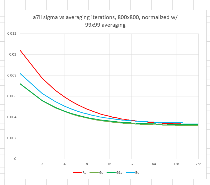
The overall PRNU is about 0.35%, and there’s no important difference between the channels.

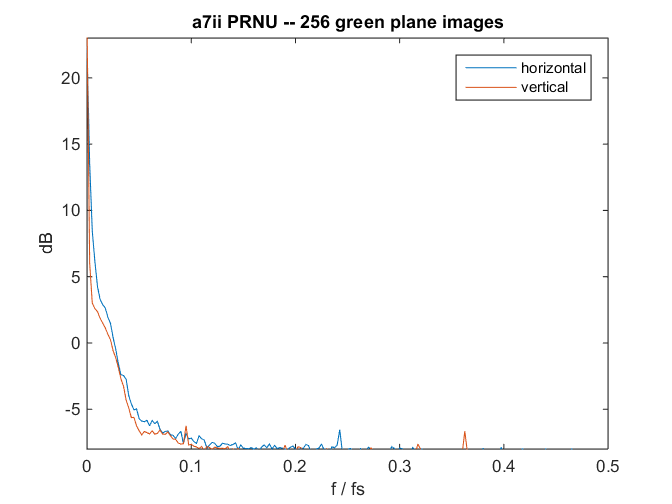
Here’s the frequency response of the first green channel of the  unfiltered version of the averaged image:
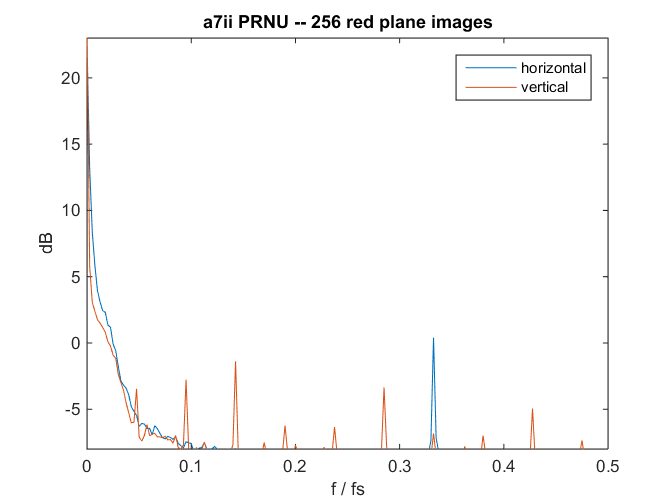
a7iifftgreen2

The red channel:

a7iifftred2

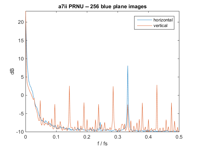
And the blue channel:

a7iifftblue2

A note about these spectra. Half the sampling frequency is on the right, and DC, or zero frequency, is on the left. The frequency scale is linear so that one octave is spread across the right half of the chart, and the next lower octave is from 1/4 to 1/2 way across the graph. The vertical axis is logarithmic, The blue horizontal frequency curve is excited by vertically oriented features in the image; and the red vertical frequency curve is excited by horizontal features in the image.

There are substantially more spiky places in the red and blue channels than in the green. Because the images were exposed under D55 illumination, the red and blue mean values are about a stop down from the green ones, and thus correction to full scale will multiply them by a larger number, but in the standard model for PRNU, that should all average out.

Here’s a histogram-equalized look at one of the green channels averaged and high pass filtered (with a 99×99 kernel) image:

AvdCorEq2

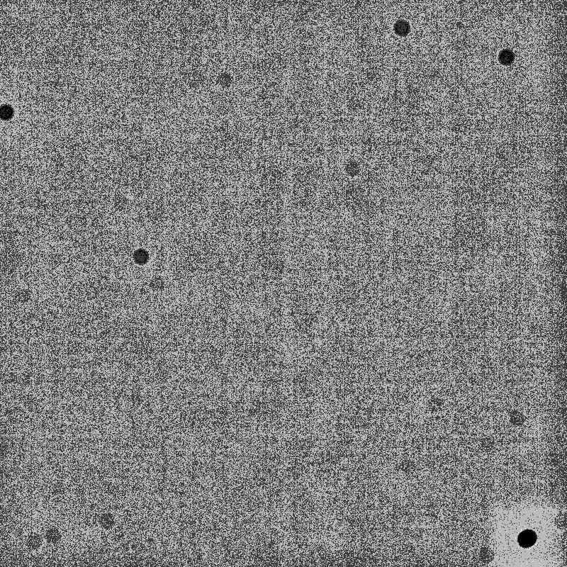
There’s quite a bit of dust for a brand new camera — I just took it out of the box, mounted a lens, and made the exposures — but it certainly won’t interfere with photography, or even be visible without the super-aggressive equalization.

Here’s the blue channel:

AvdCorEq4

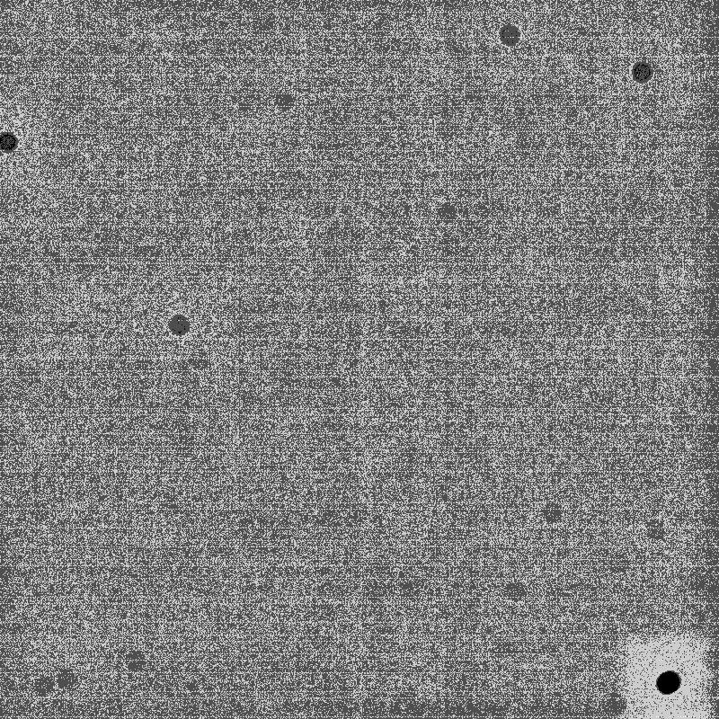
In spite of the differences in the spectra, the visual differences aren’t striking.


The Last Word

← Cleaning the data set based on SNR Modeling the a7II FWC and read noise for many ISOs →

Comments

  1. IliasG says

    December 18, 2014 at 7:19 pm

    Hi Jim,
    I am glad that you choose A7II for this round of measures 🙂

    As the PRNU looks unusually high may be it’s the on sensor PDAF pixels (half masked) the reason for this .. I mean that as these pixels receive half the light this should result in more FPN.
    It would be interesting if you could detect these pixels ..

    I found strange that for A7 (on sensor PDAF also) Bob (sensorgen) calculated from DxO data 1/3 stop less QE !!

    Reply
    • Jim says

      December 21, 2014 at 3:04 pm

      As you can see from my edit of the original post, the high PRNU was due to my misunderstanding of the way that DCRAW decoes a7II files. Fixed now.

      Jim

      Reply

Leave a Reply Cancel reply

Your email address will not be published. Required fields are marked *

May 2025
S M T W T F S
 123
45678910
11121314151617
18192021222324
25262728293031
« Apr    

Articles

  • About
    • Patents and papers about color
    • Who am I?
  • How to…
    • Backing up photographic images
    • How to change email providers
    • How to shoot slanted edge images for me
  • Lens screening testing
    • Equipment and Software
    • Examples
      • Bad and OK 200-600 at 600
      • Excellent 180-400 zoom
      • Fair 14-30mm zoom
      • Good 100-200 mm MF zoom
      • Good 100-400 zoom
      • Good 100mm lens on P1 P45+
      • Good 120mm MF lens
      • Good 18mm FF lens
      • Good 24-105 mm FF lens
      • Good 24-70 FF zoom
      • Good 35 mm FF lens
      • Good 35-70 MF lens
      • Good 60 mm lens on IQ3-100
      • Good 63 mm MF lens
      • Good 65 mm FF lens
      • Good 85 mm FF lens
      • Good and bad 25mm FF lenses
      • Good zoom at 24 mm
      • Marginal 18mm lens
      • Marginal 35mm FF lens
      • Mildly problematic 55 mm FF lens
      • OK 16-35mm zoom
      • OK 60mm lens on P1 P45+
      • OK Sony 600mm f/4
      • Pretty good 16-35 FF zoom
      • Pretty good 90mm FF lens
      • Problematic 400 mm FF lens
      • Tilted 20 mm f/1.8 FF lens
      • Tilted 30 mm MF lens
      • Tilted 50 mm FF lens
      • Two 15mm FF lenses
    • Found a problem – now what?
    • Goals for this test
    • Minimum target distances
      • MFT
      • APS-C
      • Full frame
      • Small medium format
    • Printable Siemens Star targets
    • Target size on sensor
      • MFT
      • APS-C
      • Full frame
      • Small medium format
    • Test instructions — postproduction
    • Test instructions — reading the images
    • Test instructions – capture
    • Theory of the test
    • What’s wrong with conventional lens screening?
  • Previsualization heresy
  • Privacy Policy
  • Recommended photographic web sites
  • Using in-camera histograms for ETTR
    • Acknowledgments
    • Why ETTR?
    • Normal in-camera histograms
    • Image processing for in-camera histograms
    • Making the in-camera histogram closely represent the raw histogram
    • Shortcuts to UniWB
    • Preparing for monitor-based UniWB
    • A one-step UniWB procedure
    • The math behind the one-step method
    • Iteration using Newton’s Method

Category List

Recent Comments

  • bob lozano on The 16-Bit Fallacy: Why More Isn’t Always Better in Medium Format Cameras
  • JimK on Goldilocks and the three flashes
  • DC Wedding Photographer on Goldilocks and the three flashes
  • Wedding Photographer in DC on The 16-Bit Fallacy: Why More Isn’t Always Better in Medium Format Cameras
  • JimK on Fujifilm GFX 100S II precision
  • Renjie Zhu on Fujifilm GFX 100S II precision
  • JimK on Fuji 20-35/4 landscape field curvature at 23mm vs 23/4 GF
  • Ivo de Man on Fuji 20-35/4 landscape field curvature at 23mm vs 23/4 GF
  • JimK on Fuji 20-35/4 landscape field curvature at 23mm vs 23/4 GF
  • JimK on Fuji 20-35/4 landscape field curvature at 23mm vs 23/4 GF

Archives

Copyright © 2025 · Daily Dish Pro On Genesis Framework · WordPress · Log in

Unless otherwise noted, all images copyright Jim Kasson.