This is the eighth in a series of posts on the Sony a9. The series starts here.
Note: this post has been extensively revised to correct modeling errors that result from a series of anomalies in the a9 photon transfer curves. To get around this problem, I had to prune out the data in the problem region. I don’t fully understand what’s going on, and I’ll report further as I explore the issue.
Yesterday, I looked that he fixed pattern noise (FPN) in the a9. Now I’d like to turn to the full well capacity (FWC) of the sensor. I make this test by doing pairs of exposures of a target that I’ve created for the purpose. Here’s what it looks like before I put the camera in place:
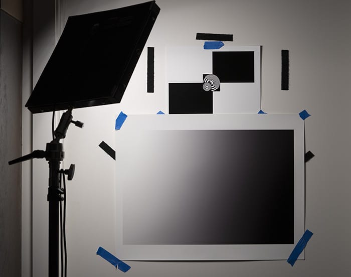
Note that the direction of the lighting is set up to follow the gradient in the target, so that I get a large range of luminance in each exposure.
Jack Hogan and I have written some Matlab code to analyze pixel response non-uniformity (PRNU) and FPN, to plot complete photon response curves, and to model sensor behavior. For all the testing except the PRNU and FPN, captures are made in pairs. By subtracting a pair of images, a image with 1.414 times the frame-independent noise, unpolluted by static noise, can be obtained, Earlier work did the captures of flat fields; one pair of images was needed for each point of the photon transfer curve (PTC). A PTC plots standard deviation versus mean value, usually using a log scale for both. While using a pair for every data point promoted accuracy, it was truly labor intensive; one set of exposures for each ISO setting for a given camera could number in the mid- thousands. This target fixes that.
You will note the absence of patches in the target. The patches are created by the software sampling the target, and they can be any convenient shape, size, and number. For the results I’m posting here, I used 12 columns and 8 rows of 200×200 pixels. The fact that the target is a gradient is not important for any single patch, since subtracting the two samples takes that out of the picture. It is important to keep the sample extents small enough that most of the sampled values are close together. That must be balanced against wanting many pixels in each sample for the purpose of having solid statistics. As it turns out, with today’s high-resolution cameras, that is no problem.
The capture protocol that I have selected is to make a set of pairs at each camera ISO setting of interest using manual exposure settings using zebras at 100+ to get the upper left corner near full scale, and varying the ISO setting. That gets the upper end of the photon transfer curves for each ISO. I also need a set of exposures nearer, but not at, the black point, which I can use to model the read noise of the camera. To get rid of quantizing artifacts, I have the program throw away samples with SNRs of less than 2, so very dark values are automatically eliminated. If the camera under test were completely ISOless, the same exposure would suffice for each dark capture, no matter what the ISO setting. My hope was that the target would have enough dynamic range so that one exposure setting would suffice even in cameras that significantly depart from ISOless behavior. So far that has worked out.
The Matlab program can model camera individually at each ISO. The program can also model a camera throughout its ISO range if it is more-or-less conventional. The a9 is not conventional, having a change in conversion gain when the ISO knob is turned from 500 to 640. Let me show you the result of both models for ISOs between 100 and 500:

I think the oddity at ISO 160 could be real, since Bill Claff has found some unusual performance there.
Here are the model values that produced the above plot.
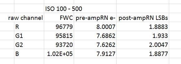
The FWC is expressed in electrons. The numbers are higher than I’ve seen for 24 MP full frame cameras, indicating that Sony continues to make better sensors. I have divided the noise contributions into two categories: those that occur before the amplifier whose gain is controlled with the ISO knob, and those that come after, including the analog-to-digital converter (ADC) itself. The pre-amp noise is expressed in the root-mean-square value in electrons, which turns out to be the same as the standard deviation. The post-amp noise is expressed in the rms value of the change in the ADC output in terms of the number of least-significant bits. The a9 has a 14-bit ADC in the mode I was testing the camera, so one LSB is one over two to the 14th power time full scale.
A useful number for sensor analysis is the unity-gain ISO, which is that ISO value which, if it existed on the ISO knob, would result in a one electron change on the sensor making a one-LSB change in the ADC output.For the a9, the unity-gain ISO is about 600. To get the total noise in LSBs from the above take the pre-amp noise above and multiply it by the ISO knob setting divided by 600, then add it in quadrature to the post-amp noise. Adding in quadrature is another way of saying take the square root of the sum of the squares. The input-referred noise in electrons is that number times 600 divided by the ISO knob setting.
If we look at the input-referred noise as modeled per-ISO, this is what we see:

Here are the FWC’s vs ISO. In a perfect world, ISO setting wouldn’t matter here:

A few nerdy words of explanation about the FWCs in the above graph. These are the full well capacities at base ISO calculated from data gathered at the ISO settings indicated on the horizontal axis. This serves as a check on the analysis software. Because of the way the a9 changes conversion gain at the ISO 500 to ISO 640 transition, to get the actual FWCs at the horizontal axis ISOs, you should divide all the FWCs at ISO 640 and above by 6.4.
Bill has suggested that maybe a better way to look at it would be to plot the number of electrons that caused the raw values to reach fullscale at each ISO. When you do that, the plot looks like this:

I slope of -1 is ideal behavior, and that’s about what we see.
Here’s the Cliff Note’s version: the a9 has impressive FWC, and pretty low, but not amazing, read noise.
Pardon my ignorance, but in practical photographic terms what does this mean? I had assumed that FWC implied a better dynamic range but a (relatively) higher noise floor means less dynamic range. Thanks for taking the time to do these tests! Looking forward to getting my A9 tomorrow and it helps to get your technical perspective to cut through the hype and hysteria.
Lower read noise as a fraction of full scale means a greater engineering dynamic range, where the noise floor limiting the dynamic range is the noise in an area of the image that receives no light at all. However, there is another source of noise in shadows that aren’t that deep, and that is the noise from the light itself. Increasing the FWC decreases the visual contribution of this kind of noise, called photon noise or shot noise, to the image. In practice, if you are particular about how much noise there is in the shadows, photon noise may be the long opole in the tent, and FWC may be more important than read noise. There is a measurement that puts both of these things together, photographic dynamic range (PDR). You can search for references here, or go to Bill Claff’s site, http://photonstophotos.net/Charts/PDR.htm.