• site home
  • blog home
  • galleries
  • contact
  • underwater
  • the bleeding edge

the last word

Photography meets digital computer technology. Photography wins -- most of the time.

You are here: Home / The Last Word / The effect of Q on sharpness

The effect of Q on sharpness

May 12, 2014 JimK 4 Comments

In the preceding few posts I explored imaging system Q, a metric for imaging system balancing. It was developed for use with monochromatic sensors and diffraction-limited optics, a luxury not enjoyed by most normal photographers. I explored the extension of the metric to cameras with Bayer color filter arrays (CFAs), with inconclusive results.

In order to gain insight as to how the concept of Q plays with Bayer CFAs, I modified a simulation that I had previously written in Matlab, adding the ability to model the diffraction of perfect lenses.

Here are the parameters I used for the simulation:

  • Perfect, diffraction-limited lens set at f/8.
  • 550 nm light used to calculate diffraction, even for the red and blue planes.
  • Kernel used for diffraction convolution 4 times as wide and tall as the Sparrow distance.
  • No vibration, no focus errors, no photon noise.
  • 14 bit perfect ADCs in the camera.
  • 100% fill factor.
  • Camera primaries are the AdobeRGB primaries.
  • Sensor dimensions are 3840 micrometers (um) x 2560 um.
  • Bilinear interpolation for demosaicing.
  • Q’s from 1 to 4. As Q goes up, the sensels get smaller, and there are more of them.

I fed the simulation a slanted edge image like this:

SlantedEdgeTgtLC

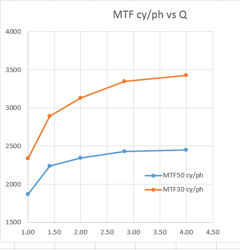
I exported the results to Imatest and had it calculate MTF50 and MTF30, the modulation transfer function values at 50% and 30% modulation. Here are those two measures of medium and lowish contrast sharpness plotted against Q:

mtfvsQ

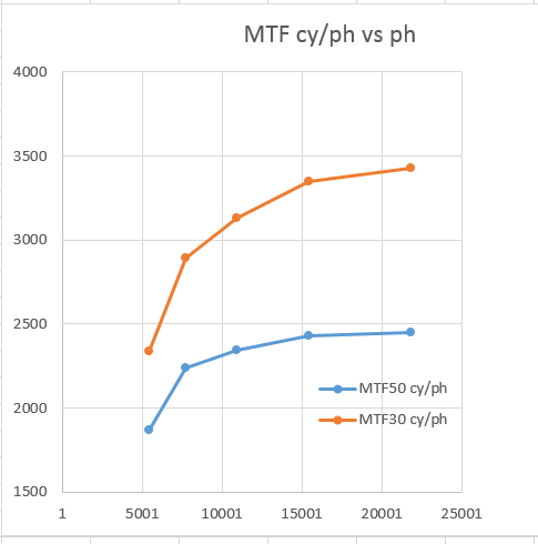
Here are the same metrics plotted against picture height in pixels for a 36x24mm (full frame) sensor:

mtfvdph

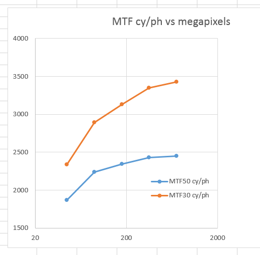
And against the number of megapixels in a 36x24mm sensor

mtfvsmp

For MTF50, by a Q of 2.8, there is no advantage in decreasing the pixel pitch for the f/8 lens. With a monochromatic sensor, that point would have occurred at Q=2. However, if we tolerate somewhat lower-contrast, there is a small advantage to be gained in going to Q=4. However, we are unlikely to see full frame cameras with a pixel pitch of 1.1 um (which is what Q=4 works out to) anytime soon.

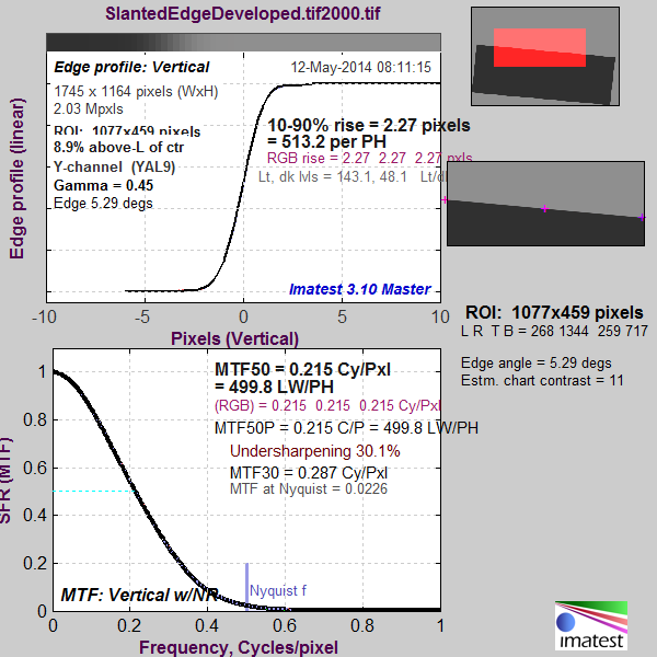
Here’s what the Imatest MTF graph looks like for a Q of 1:

SlantedEdgeDeveloped.tif1000_YA6_01_sfr

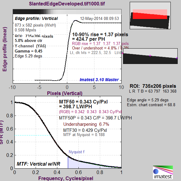
There’s quite a bit of aliasing, as shown by energy above the Nyquist frequency.

For a Q of 2, the graph looks like this:

SlantedEdgeDeveloped.tif2000_YAL9_01_sfr

You can see how the MTF in terms of cycles/pixel is going down as the Q goes up, but there are enough more pixels to make the cycles per picture height go up. There is substantially less aliasing, but there’s still some there.

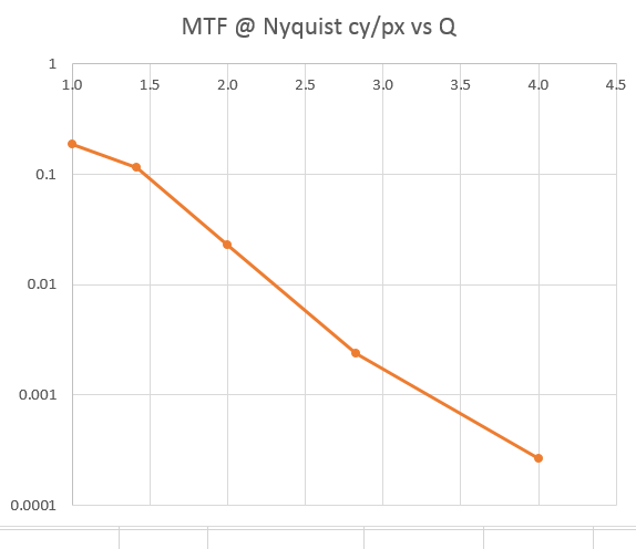
If we plot the MTF at the Nyquist frequency versus Q, which is a measure of aliasing potential, we get this:

mtfnyquist

The Last Word

← Example Q calculations for Bayer CFAs The effect of Q on false color and aliasing →

Comments

  1. Jack Hogan says

    May 13, 2014 at 8:21 am

    Hi Jim,

    Is that undershoot/overshoot in the Q=1 Edge Profile sharpening?

    Reply
    • Jim says

      May 13, 2014 at 8:42 am

      No, Jack. There was no profile. I demosaiced in Matlab using bilinear interpolation. I’m not sure why the overshoot.

      Jim

      Reply
  2. Jack Hogan says

    May 13, 2014 at 2:40 pm

    Since it’s not there in the synthetic ‘raw’ data it looks like bilinear introduces it then. Funny it’s not there in the Q=2 Edge profile.

    Reply
    • Jim says

      May 13, 2014 at 2:46 pm

      It’s something I need to look into someday. It doesn’t seem to be affecting the results in any major way. If there is a sharpening component to the demosaicing operation that I don’t understand, it’s easy to imagine that it would affect the lower-res image, which has fewer, but bigger, steps and thus more high spatial frequency information, the most.

      Jim

      Reply

Leave a Reply Cancel reply

Your email address will not be published. Required fields are marked *

May 2025
S M T W T F S
 123
45678910
11121314151617
18192021222324
25262728293031
« Apr    

Articles

  • About
    • Patents and papers about color
    • Who am I?
  • How to…
    • Backing up photographic images
    • How to change email providers
    • How to shoot slanted edge images for me
  • Lens screening testing
    • Equipment and Software
    • Examples
      • Bad and OK 200-600 at 600
      • Excellent 180-400 zoom
      • Fair 14-30mm zoom
      • Good 100-200 mm MF zoom
      • Good 100-400 zoom
      • Good 100mm lens on P1 P45+
      • Good 120mm MF lens
      • Good 18mm FF lens
      • Good 24-105 mm FF lens
      • Good 24-70 FF zoom
      • Good 35 mm FF lens
      • Good 35-70 MF lens
      • Good 60 mm lens on IQ3-100
      • Good 63 mm MF lens
      • Good 65 mm FF lens
      • Good 85 mm FF lens
      • Good and bad 25mm FF lenses
      • Good zoom at 24 mm
      • Marginal 18mm lens
      • Marginal 35mm FF lens
      • Mildly problematic 55 mm FF lens
      • OK 16-35mm zoom
      • OK 60mm lens on P1 P45+
      • OK Sony 600mm f/4
      • Pretty good 16-35 FF zoom
      • Pretty good 90mm FF lens
      • Problematic 400 mm FF lens
      • Tilted 20 mm f/1.8 FF lens
      • Tilted 30 mm MF lens
      • Tilted 50 mm FF lens
      • Two 15mm FF lenses
    • Found a problem – now what?
    • Goals for this test
    • Minimum target distances
      • MFT
      • APS-C
      • Full frame
      • Small medium format
    • Printable Siemens Star targets
    • Target size on sensor
      • MFT
      • APS-C
      • Full frame
      • Small medium format
    • Test instructions — postproduction
    • Test instructions — reading the images
    • Test instructions – capture
    • Theory of the test
    • What’s wrong with conventional lens screening?
  • Previsualization heresy
  • Privacy Policy
  • Recommended photographic web sites
  • Using in-camera histograms for ETTR
    • Acknowledgments
    • Why ETTR?
    • Normal in-camera histograms
    • Image processing for in-camera histograms
    • Making the in-camera histogram closely represent the raw histogram
    • Shortcuts to UniWB
    • Preparing for monitor-based UniWB
    • A one-step UniWB procedure
    • The math behind the one-step method
    • Iteration using Newton’s Method

Category List

Recent Comments

  • bob lozano on The 16-Bit Fallacy: Why More Isn’t Always Better in Medium Format Cameras
  • JimK on Goldilocks and the three flashes
  • DC Wedding Photographer on Goldilocks and the three flashes
  • Wedding Photographer in DC on The 16-Bit Fallacy: Why More Isn’t Always Better in Medium Format Cameras
  • JimK on Fujifilm GFX 100S II precision
  • Renjie Zhu on Fujifilm GFX 100S II precision
  • JimK on Fuji 20-35/4 landscape field curvature at 23mm vs 23/4 GF
  • Ivo de Man on Fuji 20-35/4 landscape field curvature at 23mm vs 23/4 GF
  • JimK on Fuji 20-35/4 landscape field curvature at 23mm vs 23/4 GF
  • JimK on Fuji 20-35/4 landscape field curvature at 23mm vs 23/4 GF

Archives

Copyright © 2025 · Daily Dish Pro On Genesis Framework · WordPress · Log in

Unless otherwise noted, all images copyright Jim Kasson.