The joys and difficulties of modern instrumentation

This is an aside to a  series of posts on power consumption in the Sony a7RII. The more recent incarnation of the series starts here.

I was recently surprised by one of the scope traces that I made as part of the a7RII current draw tests:

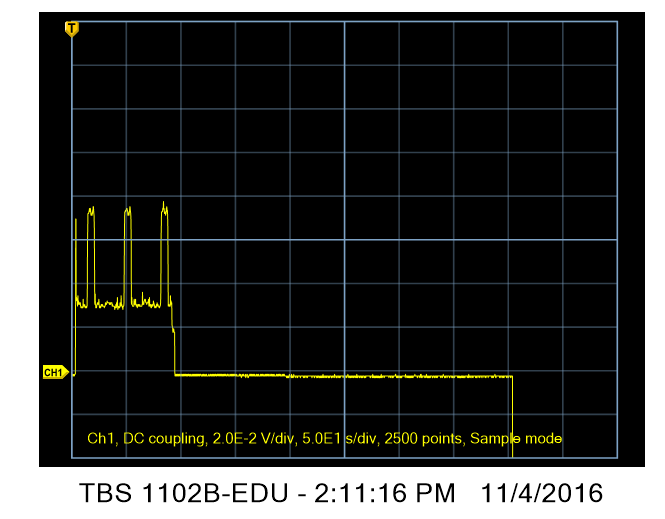
I turned on the camera at the far left of the trace, which has a time base of 50 seconds per division. I left it on for about a minute and a half, then I turned it off. You can see the current drop suddenly, and — if you’ve got good eyes — drop again after the camera has been off for a minute or so. But there’s something that is clearly not right. Look at those large variations in current when the camera is on. That can’t be, can it? 

Of course it can’t. I’ll explain further down the page.

But first, let me reminisce about oscilloscopes. The first scope that I used when I was a electronics technician in a summer job while I was an EE undergrad at Stanford, was an hp 120. It was truly a dog of a scope: slow, limited in features, and unsophisticated in its triggering. Its only saving grace was that it was cheap, at least by hp standards (later on, I worked for hp, and we used to say to each other “the quality goes in before the price goes on” in a parody of an advertising slogan of the day). After I got my MSEE, I returned to the same company, and got a better scope: a midline Tektronix. After a couple of years, when I was running research projects, I bought (with company money) myself my dream scope, a Tektronix 547, and two plugins, a 4-channel single ended one for digital work, and a two channel differential one for analog stuff. The 547 used tubes (and transistors, too), so in a sense it wasn’t the state of the art. But man-oh-man, it was a sweet piece of gear. 50 MHz bandwidth (100 times the hp 120), great triggering, controls that looked like the flight deck of a 707 (this was in about 1967), and precision bbuilt into every nook and cranny.

I loved that scope. It was the high water mark of my scope ownership (OK, OK, I didn’t really own it, but I was sure possessive). When I went to hp, they tried to stick me with another 120, but I cried foul and got a 180, which wasn’t a bad scope, but — to paraphrase Lloyd Bentsen — it was no 547.

I had plenty of nice gear to use at hp and later on at Rolm, but I’ll always have a soft spot in my heart for that Tek 547. 

In order to do the dynamic current draw analyses that I’ve been reporting on, I purchased a modern Tektronix scope, a TBS 1102B.  Definitely not the high-end device that the 547 was, it cost less than a twentieth of the older scope price in inflation-adjusted dollars, and in most every way outperforms it wildly. It’s got twice the bandwidth (but only two channels, although I could have had four if I wanted to pony up for that version). It connects to a computer — goodbye scope camera. It’s got numerical measurement and calculation capability built in. You can pick it up easily in one hand (the 547 weighed more than 70 pounds, not counting the obligatory cart and scope camera). It’s just a better product. 

But all that comes a a small price. The controls feel lousy by comparison. And the scope can mislead you if you’re not paying attention. 

Here’s a trace with another instrument (a Keithley 2100 DMM) of a similar shutdown on the same camera:

The odd variations in current when the camera is one are replaced by pseudo-random cycling between two current values.

Neither one is right. And they’re both wrong for the same reason: aliasing. 

The scope’s time base was set to 50 seconds/division. The scope samples the input signal 2500 times in a sweep, or 500 times in the 50 seconds that it takes to travel one division horizontally. That’s 10 samples per second, or a sample every 100 milliseconds. However, the camera is changing the current about 30 times a second, and there’s only a 10 microsecond RC filter in front of the scope. So the variations in the current that we’re seeing in the scope trace at the beginning of this post are a result of the sampling frequency of the scope and the refresh frequency of the camera beating against each other.

In the old days, there were special-purpose scopes called sampling scopes that we used for very high speed measurements. We had a saying” “Sampling scopes lie.” Now all new scopes are sampling scopes.