What’s MTF50 = x look like: sim pix

Last week, I wrote this post on producing images that show visually the effect of image capture blur on Bayer-CFA cameras. I briefly discussed this simulation-based approach:

Start out with a slanted edge. Dial in some diffraction, some motion blur, some defocusing, take the captured image, run it through a slanted edge analyzer, and get the MTF50. The, leaving the simulator settings the same, run a natural world photograph through the simulator. Do that with various simulated camera blur, and we’ll get a series of images that people can look at, and we’ll know their MTF50.

I went on to discuss ways to do similar captures with real, not simulated cameras. I’ve decided to pursue the simulator approach. It allows me to have identical scenes with different amounts and kinds of camera blur, and give me great freedom in the kinds of input images that I use.

However, there is a technical problem. Because of the way the simulator works, it needs an image of at least 8 times the linear resolution of the output image for accurate results at MTF50s of over 1000 cycles/picture height. That means that it’s not practical for me to simulate the entire capture of a full-frame camera, but only a crop from that capture. Even then, I need to go to extraordinary lengths to get sufficiently high resolution in my input images.

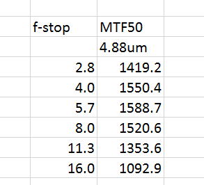
Let’s work through an example. I first computed MTF50 values for with pixel pitch set to 4.88 um (same as a7R or D800 or D810), and a simulated Zeiss Otus lens, at f/2.8 through f/16.

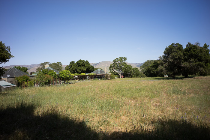
I set up on this scene, shown captured by a 24mm lens (Leica 24mm f/3.4 Elmar-M ASPH, if you care) on a Sony a7II:

Then I put a Leica 180mm f/3.4 Apo-Telyt on the camera, focused manually, set the aperture to f/8, and made a three-row series of exposures. I stitched them in AutoPano Giga, and got this 14825×8037 pixel result:

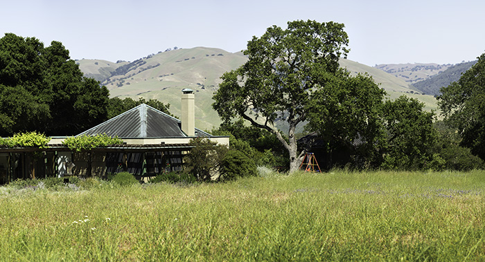
Consider it a crop from the full frame first image represented by the 24mm picture.

Then I ran the 14825×8037 image through the camera simulator with pixel pitch set to 4.88 um (same as a7R or D800 or D810), and a simulated Zeiss Otus lens, at f/2.8 through f/16. I set the reduction factor to 8, so the resulting images were 1853×1005 pixels. Note that the ratio between the focal length I used for the pano is about eight times the 24mm lens I used for the overall FF shot; that’s the same as the reduction ratio.

I made some 1:1 crops from the images, and blew them up to 300% just like I do when I’m doing lens testing.

I didn’t include the f/2.8, f/4, and f/8 images because they were so similar to the f/5.6 one.

The real test of what sharpness is acceptable for printing is to make some test prints. Therefore, I encourage anyone who wants to know what 36MP prints with MTF50s between 1000 cycles/picture height or so and 1600 cycles/picture height or so download the files,  resize them — without resampling! — to your printer’s native driver resolution (360 ppi for Epsons, 300 ppi for Canons) and print them. Then look at them to find what is your own personal minimum acceptable sharpness. Note the f-stop. Now go to the table above and note the MTF50 associated with that f-stop. Congratulations! You’ve just found your minimum acceptable MTF50.

Note that I’m using gradient-corrected linear interpolation, which is not the most sophisticated demosaicing algorithm in the world.

Comments and questions are welcome.