the last word

Photography meets digital computer technology. Photography wins -- most of the time.

  • site home
  • blog home
  • galleries
  • contact
  • underwater
  • the bleeding edge
You are here: Home / a7RIII / a7RIII star-eater green channel histograms

a7RIII star-eater green channel histograms

November 22, 2017 JimK 7 Comments

This is the sixth in a series of posts on the Sony a7RIII (and a7RII, for comparison) spatial processing that is invoked when you use a shutter speed of longer than 3.2 seconds. The series starts here.

A reader made this comment to an earlier post.

My analysis of raw files and the “pixel pairing” artifact suggests an important difference between the v3.3 and v4.0 algorithms. Green pixels are far more likely to survive the v4.0 algorithm. So the green parts of a small star survive and the star remains visible.

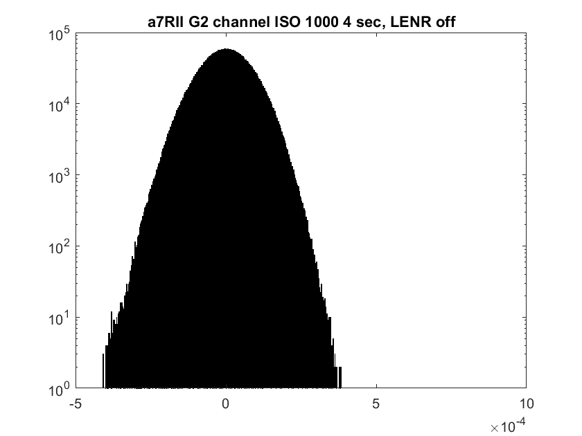
I had only been looking at red channel histograms, so now I’m turning my attention to the green channels.

You’ll note that I’ve fixed the scaling of the horizontal axes in these plots to the same limits.


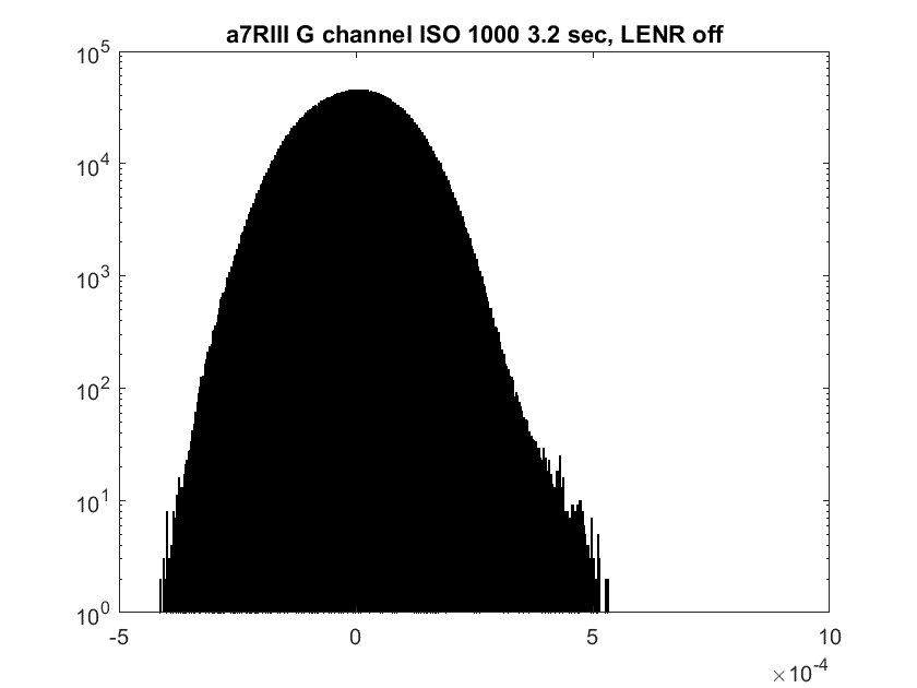
The reduction in the upper tail of the distribution is apparent, so the a7RIII version is pretty aggressive.

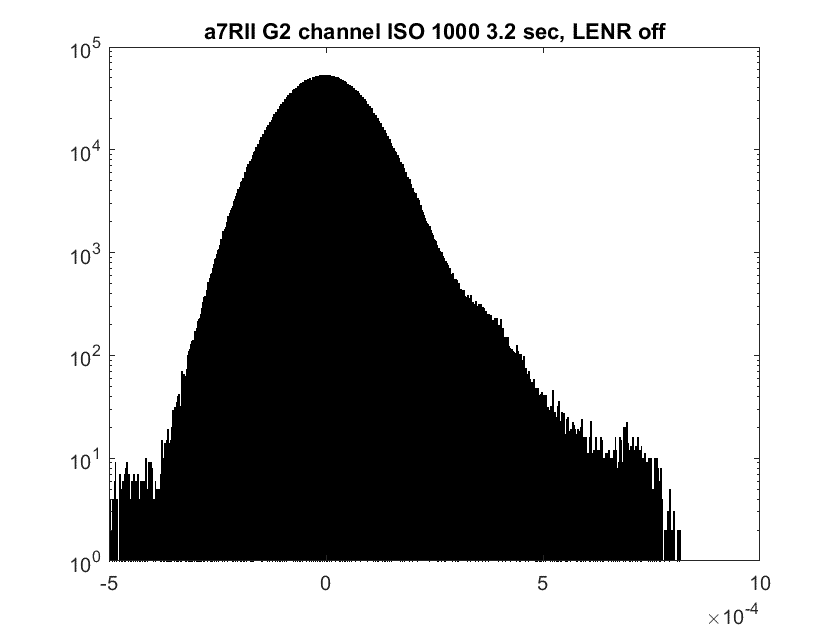
The a7RII has a bigger spread before the hot-pixel algorithm kicks in.

But the outliers appear to be reduced by more. So maybe there is some difference.

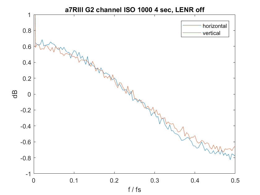
Here are the G2 channes, just for completeness.


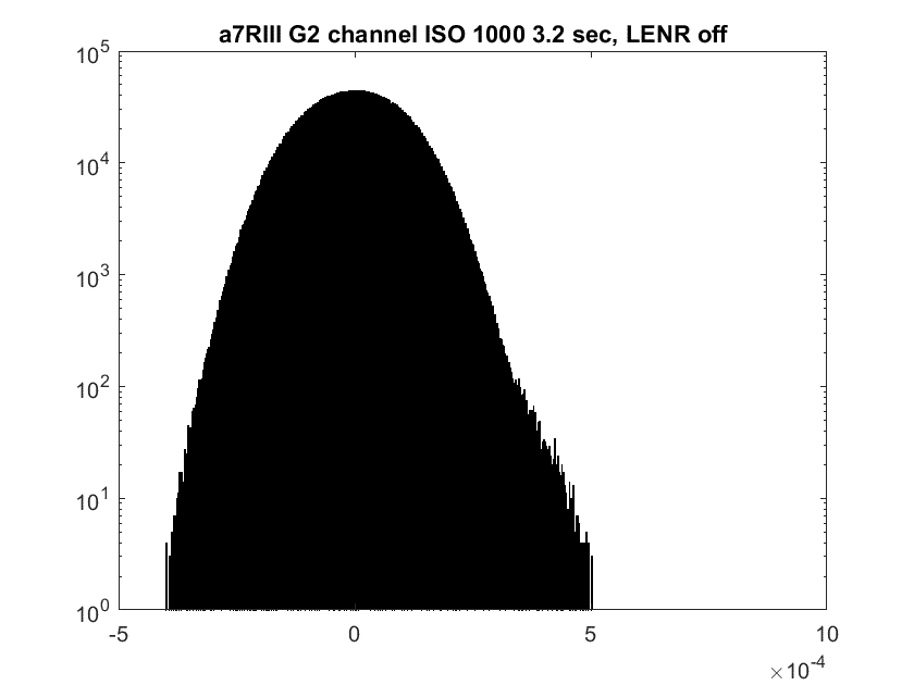
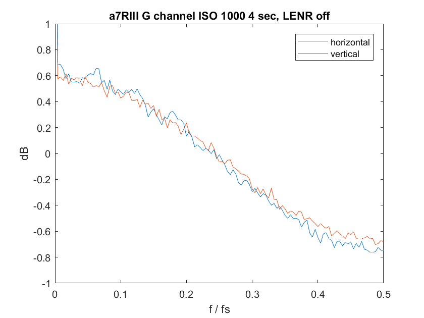
If we look at the green channel frequency plots, they look like what we saw with the red channel.


a7RIII

← a7RII star-eating histograms Testing for a7RIII star-eating by direct search →

Comments

  1. Mark Shelley says

    November 22, 2017 at 10:03 pm

    Hi Jim. I think that in the end only a detailed examination of the image at the pixel level will show the difference between the algorithms. I’m on the road at present but if you Google search my page “diagnosing star eater” you will find it all explained there, including what I mean by “pixel pairing”.

    Reply
    • JimK says

      November 23, 2017 at 8:06 am

      Mark, there is excellent material on your site, but I am a loss as to how to turn it into a code that measures the effect. Maybe you can give me some ideas when you return home.

      Reply
      • Mark Shelley says

        November 24, 2017 at 3:38 am

        Sure, after the weekend. You might find some useful info here from a previous discussion: https://www.dpreview.com/forums/post/59693566

        Reply
    • JimK says

      November 23, 2017 at 8:07 am

      In your post on pairing, you show the results of testing with artificial stars. Would it be easy for me to create an artificial star target? If so, can you provide some advice? It’s difficult for me to get more than 25 feet away, so getting a small aperture would be important. I see that there are commercial units, but some don’t specify apertures, and others seem to have ones that are too large. I’m figuring a 80 mm lens at 8 meters would be a 100:1 reduction ratio, and to get the star smaller than the pitch, I’d need the artificial star to be 450 um, or 0.45 mm in diameter. And that’s without defocus, aberrations, and diffraction.

      Added: I see the Hubble star simulator has apertures as small as 50 um. That sounds good. I’m going to order one.

      Reply
      • Mark Shelley says

        November 24, 2017 at 3:12 am

        Mine was DIY – battery torch covered in baking foil with tiniest pinprick and placed at sufficient distance in the dark. Hubble one looks good. It’s certainly the key to “before” and “after” repeatable experiments.

        Reply
    • JimK says

      November 23, 2017 at 9:10 am

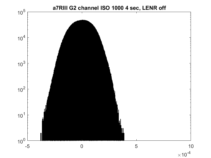
      It is clear from these gross histograms that green channel outliers are being removed in the 4-second exposures, though.

      Reply
      • Mark Shelley says

        November 23, 2017 at 10:36 am

        When I said green pixels are more likely to survive, I meant only within a small star. In random data there will be no observed difference.

        Reply

Leave a Reply Cancel reply

Your email address will not be published. Required fields are marked *

March 2023
S M T W T F S
 1234
567891011
12131415161718
19202122232425
262728293031  
« Jan    

Articles

  • About
    • Patents and papers about color
    • Who am I?
  • Good 35-70 MF lens
  • How to…
    • Backing up photographic images
    • How to change email providers
  • Lens screening testing
    • Equipment and Software
    • Examples
      • Bad and OK 200-600 at 600
      • Excellent 180-400 zoom
      • Fair 14-30mm zoom
      • Good 100-200 mm MF zoom
      • Good 100-400 zoom
      • Good 100mm lens on P1 P45+
      • Good 120mm MF lens
      • Good 18mm FF lens
      • Good 24-105 mm FF lens
      • Good 24-70 FF zoom
      • Good 35 mm FF lens
      • Good 60 mm lens on IQ3-100
      • Good 63 mm MF lens
      • Good 65 mm FF lens
      • Good 85 mm FF lens
      • Good and bad 25mm FF lenses
      • Good zoom at 24 mm
      • Marginal 18mm lens
      • Marginal 35mm FF lens
      • Mildly problematic 55 mm FF lens
      • OK 16-35mm zoom
      • OK 60mm lens on P1 P45+
      • OK Sony 600mm f/4
      • Pretty good 16-35 FF zoom
      • Pretty good 90mm FF lens
      • Problematic 400 mm FF lens
      • Tilted 20 mm f/1.8 FF lens
      • Tilted 30 mm MF lens
      • Tilted 50 mm FF lens
      • Two 15mm FF lenses
    • Found a problem – now what?
    • Goals for this test
    • Minimum target distances
      • MFT
      • APS-C
      • Full frame
      • Small medium format
    • Printable Siemens Star targets
    • Target size on sensor
      • MFT
      • APS-C
      • Full frame
      • Small medium format
    • Test instructions — postproduction
    • Test instructions — reading the images
    • Test instructions – capture
    • Theory of the test
    • What’s wrong with conventional lens screening?
  • Previsualization heresy
  • Privacy Policy
  • Recommended photographic web sites
  • Using in-camera histograms for ETTR
    • Acknowledgments
    • Why ETTR?
    • Normal in-camera histograms
    • Image processing for in-camera histograms
    • Making the in-camera histogram closely represent the raw histogram
    • Shortcuts to UniWB
    • Preparing for monitor-based UniWB
    • A one-step UniWB procedure
    • The math behind the one-step method
    • Iteration using Newton’s Method

Category List

Recent Comments

  • Mal Paso on Christmas tree light bokeh with the XCD 38V on the X2D
  • Sebastian on More on tilted adapters
  • JimK on On microlens size in the GFX 100 and GFX 50R/S
  • Kyle Krug on On microlens size in the GFX 100 and GFX 50R/S
  • JimK on Hasselblad X2D electronic shutter scan time
  • Jake on Hasselblad X2D electronic shutter scan time
  • Piotr Chylarecki on Who am I?
  • JimK on Who am I?
  • Piotr Chylarecki on Who am I?
  • Stefan on Swebo TC-1 OOBE

Archives

Copyright © 2023 · Daily Dish Pro On Genesis Framework · WordPress · Log in

Unless otherwise noted, all images copyright Jim Kasson.