• site home
  • blog home
  • galleries
  • contact
  • underwater
  • the bleeding edge

the last word

Photography meets digital computer technology. Photography wins -- most of the time.

You are here: Home / GFX 100S / Predicting lower-contrast MTFxx from MTF50

Predicting lower-contrast MTFxx from MTF50

June 14, 2021 JimK 4 Comments

This is one in a series of posts on the Fujifilm GFX 100S. You should be able to find all the posts about that camera in the Category List on the right sidebar, below the Articles widget. There’s a drop-down menu there that you can use to get to all the posts in this series; just look for “GFX 100S”.

After I published this post, I got a bit of pushback from a reader. His contention was that DOF is defined by low-contrast portions of the image, and by measuring MTF50, I was looking at high-contrast areas. I don’t buy the premise, but I thought it worthwhile to take a look at the ability of MTF50 to predict the behavior of lower-contrast MTFxx’s, like MTF20 or MTF10.

I took the through-focus tests that I did of the Fujifilm 80 mm f/1.7 GF and the 110 mm f/2 GF lenses on the GFX 100S and created scatter plots of MTF10 versus MTF50 for all the images. I didn’t do any fancy curve-fitting, so the data jumps around due to the vicissitudes of the GFX focus bracketing system, but it’s enough to get the idea. There is also no interpolation, so both sets of data are rather coarsely quantized. At wide apertures, the 110 and the 80 both have different MTF curves when they are front-focused and when they are back-focused. In order to make that easier to sort out, I colored the front-focused points red and the back-focused points blue. The coloring isn’t perfect, but, again, it’s good enough to get the idea.

Without further ado, here are the plots, first at f/2:

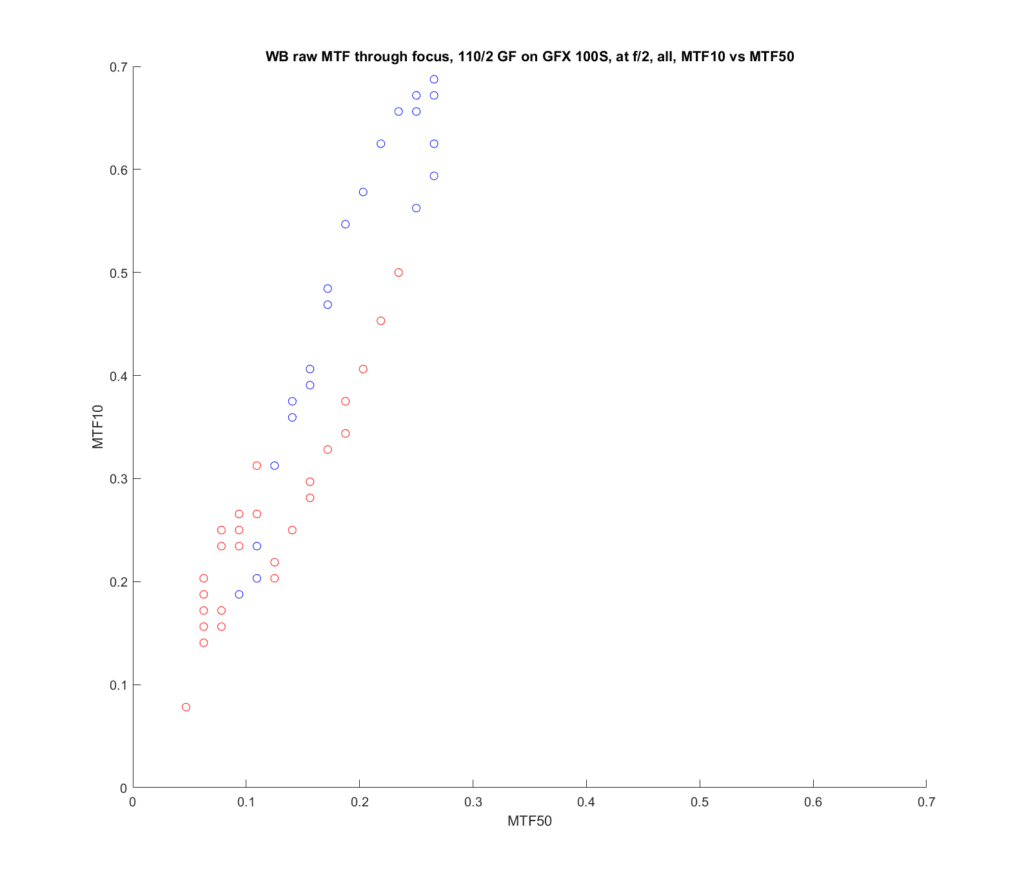
MTF50, in cycles per pixel, is plotted on the x axis, and MTF10, also in cycles per pixel, is on the y axis.

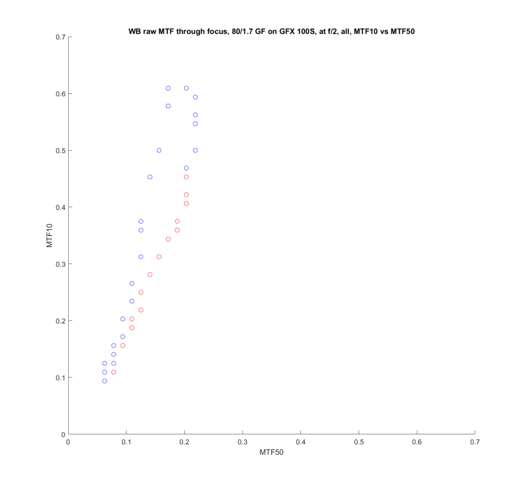
There is strong correlation of MTF10 to MTF 50, but, for the saem MTF50 values, the MTF10 values are higher when the lens is back-focused than when it is front-focused. This means that there is relatively more low-contrast detail when the lens is back-focused. Even though the 110/2 and the 80/1.7 are quite different designs, with the 110 being better corrected, the effect appears for both lenses. The effect occurs most strongly at high MTF50. When the MTF 50 is down around 0.15 cycles per pixel, it hardly exists at all.

You should take the MTF10 numbers above 0.5 with a whole box of salt. Half a cycle per pixel is the Nyquist frequency, and any information captured above that frequency will be improperly reconstructed in the photograph.

Stopping down to f/2.8:

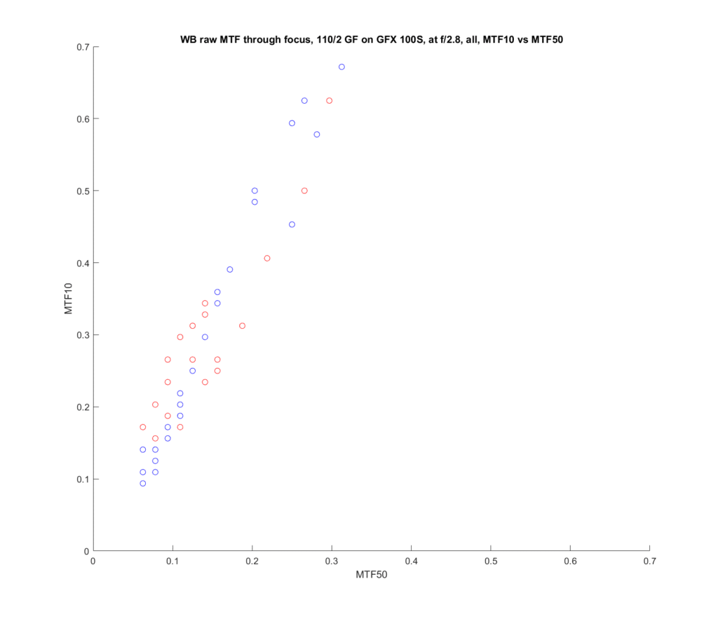
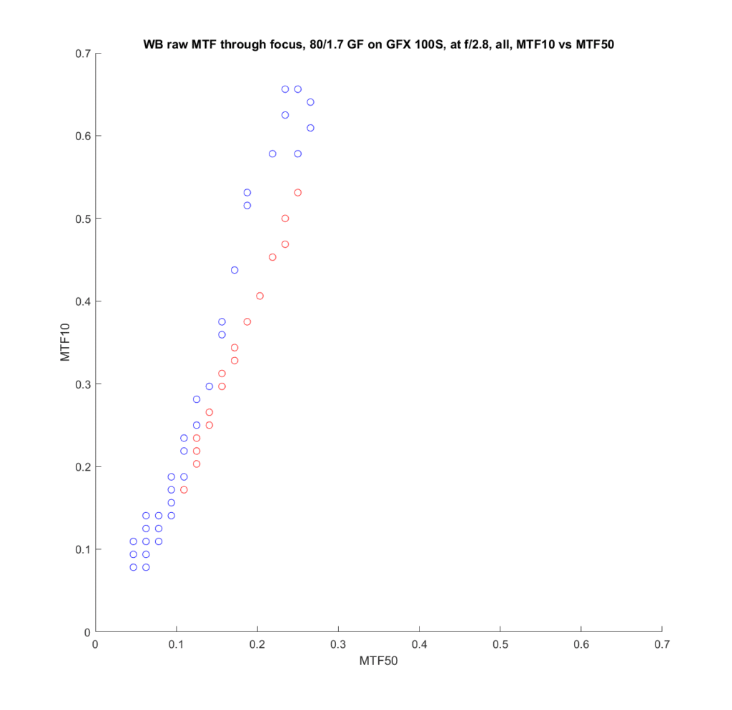
In both cases, the effect is reduced, and hardly exists at MTF50s below 0.2 cycles per pixel.

At f/4:


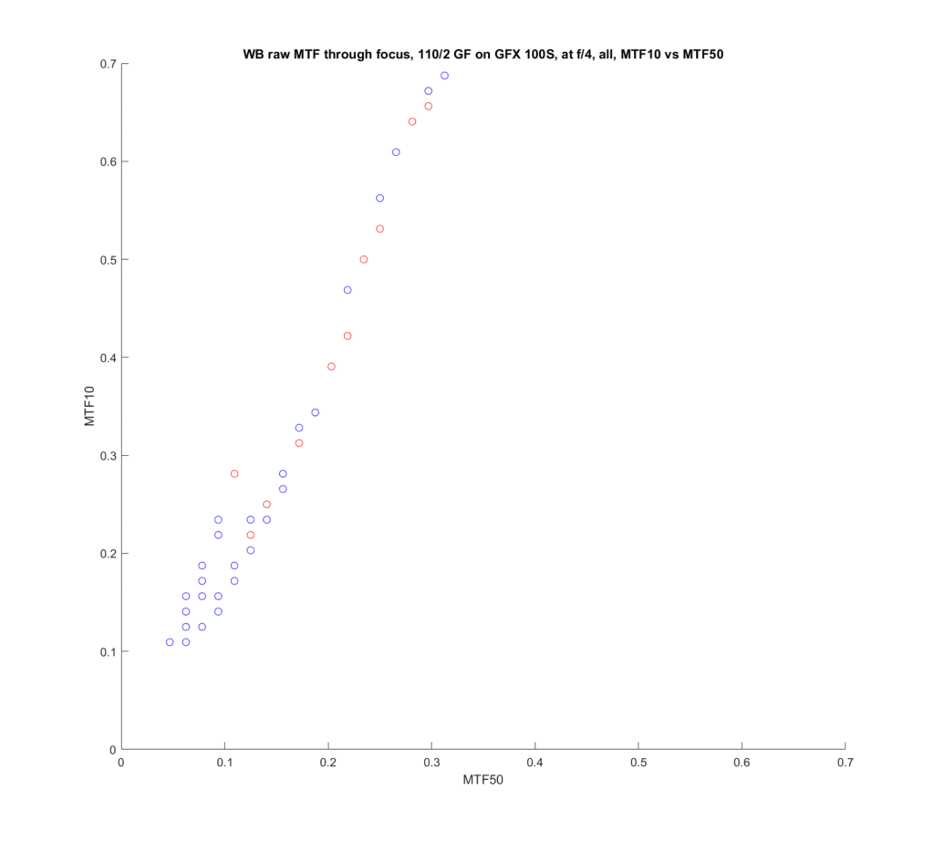
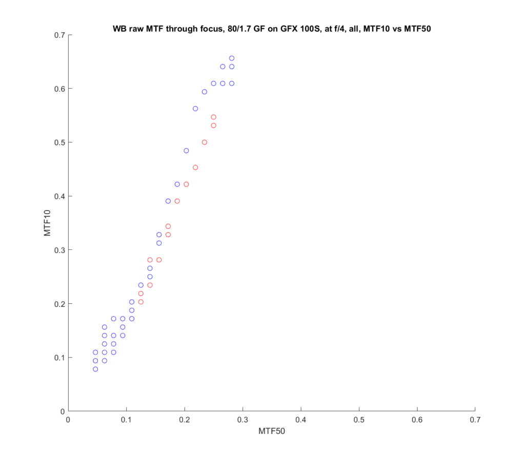
The effect is almost gone.

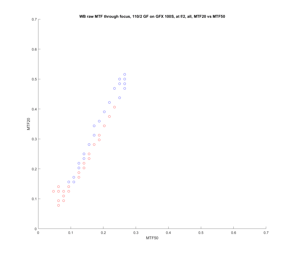
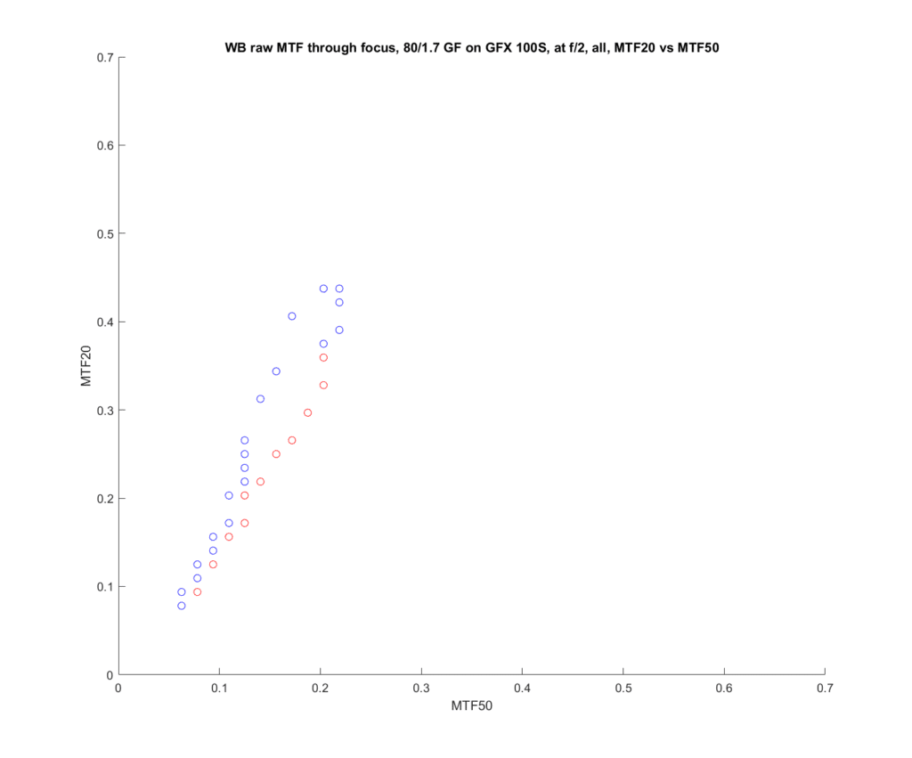
I plotted similar curves for MTF20 vs MTF 50, and they looked roughly the same, but the asymmetry around the correct focus was smaller, especially with the 110/2.

Here are the f/2 plots:


I think I’ll continue to use MTF50 for these tests. However, I’m working on ways to present the entire MTF curve for these through focus tests.

Here’s a teaser:


GFX 100S

← Copying watercolors with the GFX 100 Displaying transfocal MTF curves →

Comments

  1. David Berryrieser says

    June 14, 2021 at 10:55 am

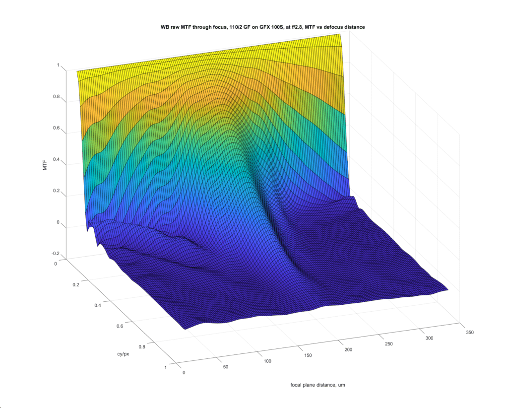
    I seriously doubt anyone could tell the difference between the DOF characteristics of the real image and one approximated using a linear fit between the MTF10 and MTF50 shown above, assuming LOCA and everything else were kept the same. I suspect that the relationship to higher contrast levels would be even better. For defocus at least, I am convinced that MTF50 provides a good scalar metric for most of the MTF.

    It would be fun to see the full MTF curve vs defocus. Time to pull out a 3D plot? Color scale a 2D image of the data?

    Reply
    • JimK says

      June 14, 2021 at 11:19 am

      It would be fun to see the full MTF curve vs defocus.

      Working on it. It looks pretty ugly with the raw data. I’ll see if I can apply the same smoothing algorithm I used before.

      Reply
      • Brandon Dube says

        June 14, 2021 at 12:27 pm

        It would be good for you to replicate figure 34 from my thesis, and fig 37 if you try to do any model fitting. https://www.retrorefractions.com/pdf/bdd_ug_thesis_10.pdf

        Reply
        • JimK says

          June 14, 2021 at 12:33 pm

          Thanks, Brandon. I was thinking either something like that, a 3D surface, or a contour plot. But I’ve got to smooth the data first.

          Reply

Leave a Reply Cancel reply

Your email address will not be published. Required fields are marked *

May 2025
S M T W T F S
 123
45678910
11121314151617
18192021222324
25262728293031
« Apr    

Articles

  • About
    • Patents and papers about color
    • Who am I?
  • How to…
    • Backing up photographic images
    • How to change email providers
    • How to shoot slanted edge images for me
  • Lens screening testing
    • Equipment and Software
    • Examples
      • Bad and OK 200-600 at 600
      • Excellent 180-400 zoom
      • Fair 14-30mm zoom
      • Good 100-200 mm MF zoom
      • Good 100-400 zoom
      • Good 100mm lens on P1 P45+
      • Good 120mm MF lens
      • Good 18mm FF lens
      • Good 24-105 mm FF lens
      • Good 24-70 FF zoom
      • Good 35 mm FF lens
      • Good 35-70 MF lens
      • Good 60 mm lens on IQ3-100
      • Good 63 mm MF lens
      • Good 65 mm FF lens
      • Good 85 mm FF lens
      • Good and bad 25mm FF lenses
      • Good zoom at 24 mm
      • Marginal 18mm lens
      • Marginal 35mm FF lens
      • Mildly problematic 55 mm FF lens
      • OK 16-35mm zoom
      • OK 60mm lens on P1 P45+
      • OK Sony 600mm f/4
      • Pretty good 16-35 FF zoom
      • Pretty good 90mm FF lens
      • Problematic 400 mm FF lens
      • Tilted 20 mm f/1.8 FF lens
      • Tilted 30 mm MF lens
      • Tilted 50 mm FF lens
      • Two 15mm FF lenses
    • Found a problem – now what?
    • Goals for this test
    • Minimum target distances
      • MFT
      • APS-C
      • Full frame
      • Small medium format
    • Printable Siemens Star targets
    • Target size on sensor
      • MFT
      • APS-C
      • Full frame
      • Small medium format
    • Test instructions — postproduction
    • Test instructions — reading the images
    • Test instructions – capture
    • Theory of the test
    • What’s wrong with conventional lens screening?
  • Previsualization heresy
  • Privacy Policy
  • Recommended photographic web sites
  • Using in-camera histograms for ETTR
    • Acknowledgments
    • Why ETTR?
    • Normal in-camera histograms
    • Image processing for in-camera histograms
    • Making the in-camera histogram closely represent the raw histogram
    • Shortcuts to UniWB
    • Preparing for monitor-based UniWB
    • A one-step UniWB procedure
    • The math behind the one-step method
    • Iteration using Newton’s Method

Category List

Recent Comments

  • bob lozano on The 16-Bit Fallacy: Why More Isn’t Always Better in Medium Format Cameras
  • JimK on Goldilocks and the three flashes
  • DC Wedding Photographer on Goldilocks and the three flashes
  • Wedding Photographer in DC on The 16-Bit Fallacy: Why More Isn’t Always Better in Medium Format Cameras
  • JimK on Fujifilm GFX 100S II precision
  • Renjie Zhu on Fujifilm GFX 100S II precision
  • JimK on Fuji 20-35/4 landscape field curvature at 23mm vs 23/4 GF
  • Ivo de Man on Fuji 20-35/4 landscape field curvature at 23mm vs 23/4 GF
  • JimK on Fuji 20-35/4 landscape field curvature at 23mm vs 23/4 GF
  • JimK on Fuji 20-35/4 landscape field curvature at 23mm vs 23/4 GF

Archives

Copyright © 2025 · Daily Dish Pro On Genesis Framework · WordPress · Log in

Unless otherwise noted, all images copyright Jim Kasson.