• site home
  • blog home
  • galleries
  • contact
  • underwater
  • the bleeding edge

the last word

Photography meets digital computer technology. Photography wins -- most of the time.

You are here: Home / GFX 100 / Off-axis testing of the Fuji 45/2.8 and 50/3.5 GF on the GFX 100S

Off-axis testing of the Fuji 45/2.8 and 50/3.5 GF on the GFX 100S

July 7, 2021 JimK Leave a Comment

This is one in a series of posts on the Fujifilm GFX 100S. You should be able to find all the posts about that camera in the Category List on the right sidebar, below the Articles widget. There’s a drop-down menu there that you can use to get to all the posts in this series; just look for “GFX 100S”. Since it’s more about the lenses than the camera, I’m also tagging it with the other Fuji GFX tags.

In the previous six posts, I tested the off axis performance of the Fujifilm 110 mm f/2, 80 mm f/1.7 , 250 mm f/4, 63 mm f/2.8, 45 mm f/2.8, and 120 mm f/4 macro GF lenses on a GFX 100S. Now I’ll do the same with the 50mm f/3.5 lens. Since there’s been a lot of interest in comparing the 45 and the 50 mm GF lenses, I’ll include information on the 45 here, to9.

Here’s the test protocol:

  • RRS carbon fiber legs
  • C1 head
  • Target distance 4 meters for 45  mm lens
  • Target distance 4.4 meters for 50 mm lens
  • ISO 100
  • Electronic shutter
  • 10-second self timer
  • f/2.8 through f/11 in whole-stop steps for the 45
  • f/4 through f/11 in whole-stop steps for the 50
  • Exposure time set by camera in A mode
  • Focus bracketing, step size 1, 120 to 60 exposures
  • Initial focus well short of target
  • Convert RAF to DNG using Adobe DNG Converter
  • Extract raw mosaics with dcraw (I’ll change this to libraw and drop the DNG conversion when I get the chance, but the Matlab program  that controls all this is written for dcraw)
  • Extract slanted edge for each raw plane in a Matlab program the Jack Hogan originally wrote, and that I’ve been modifying for years.
  • Analyze the slanted edges and produce MTF curves using MTF Mapper (great program; thanks, Frans)
  • Fit curves to the MTF Mapper MTF50 values in Matlab
  • Correct for systematic GFX focus bracketing inconsistencies
  • Analyze and graph in Matlab

I analyzed a horizontal edge in the center of the frame, and both a horizontal and a vertical edge on the far right side of the frame. The horizontal edge is oriented in a radial direction, and that’s how I’m identifying it in the plots. The horizontal edge is oriented in a tangential direction, and that’s the way I’m tagging it. I also redid the tests with the target on the lens axis.  I looked at both horizontal and vertical edges. The edges are identified on the graphs as, respectively,  radial and tangential edges. Those terms don’t make sensor on axis. The numbers ought to be the same.

Here are the MTF50 results for the 45 and the 50, in cycles per picture height:

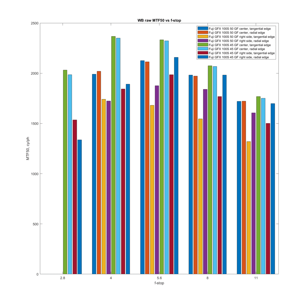
I measured the MTF50 on each of the raw channels, and am reporting on the MTF50 on a white-balanced composite of those channels, which is mostly the green channel. The 50 doesn’t get a lot on internet respect, but it’s not far off the 45 here.

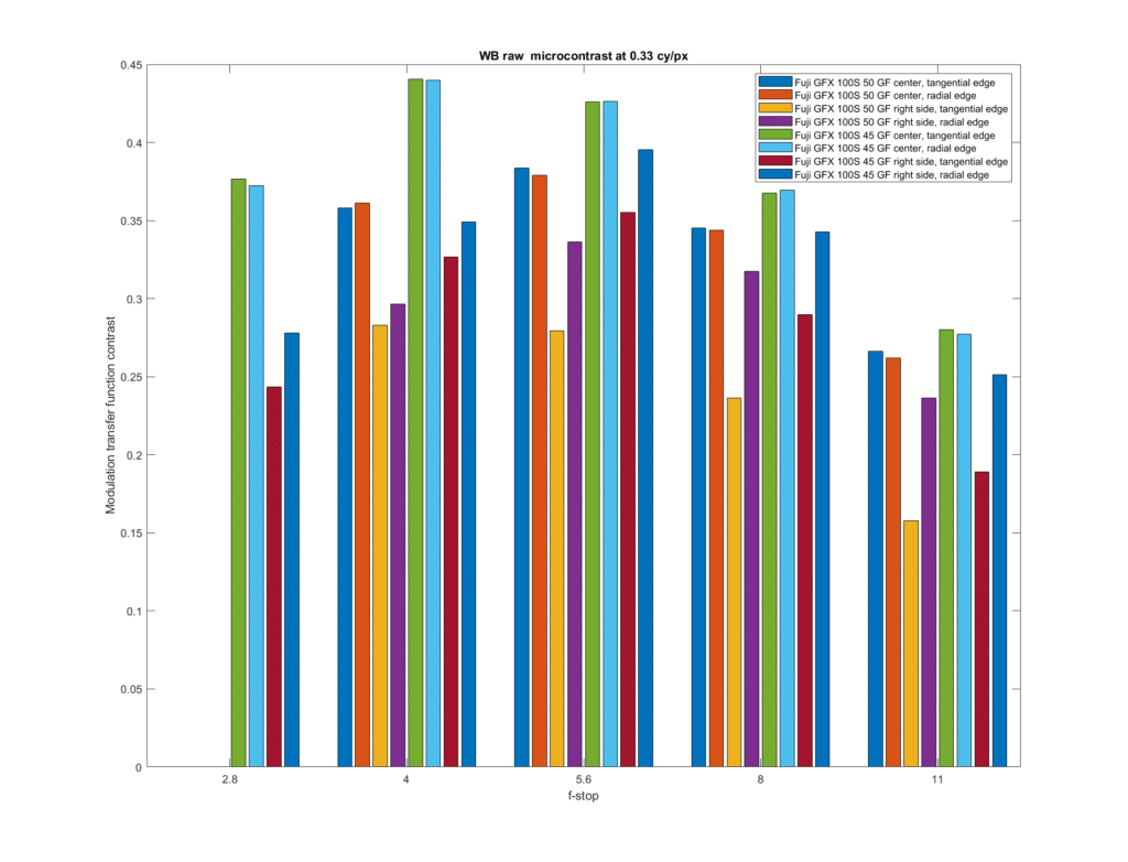
Here is the microcontrast at 0.33 cycles per pixel.

Now we’ll look at longitudinal chromatic aberration (LoCA).

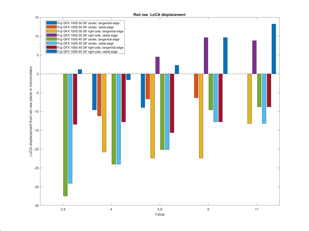
The above plots the shift of the red raw image plane (on the sensor side of the lens) compared to the white-balanced raw plane. If anything, the 50 has less LoCA than the 45.

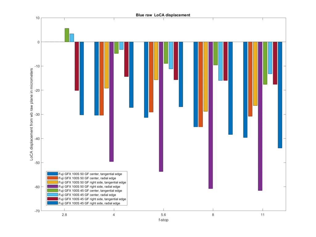
The blue LoCA for the 50 is greater.

Now we’ll look at some transfocal bokeh images.

45, f/4, center


50, center, f/4


50, right side, radial edge, f/4


45, f/4, right side, radial edge


50, right side, tangential edge, f/4


45, f/4, right side, tangential edge


GFX 100, GFX 100S, GFX 50S

← Off-axis testing of the Fuji 45/2.8 GF on the GFX 100S Off-axis testing of the Fuji 30/3.5 GF on the GFX 100S →

Leave a Reply Cancel reply

Your email address will not be published. Required fields are marked *

May 2025
S M T W T F S
 123
45678910
11121314151617
18192021222324
25262728293031
« Apr    

Articles

  • About
    • Patents and papers about color
    • Who am I?
  • How to…
    • Backing up photographic images
    • How to change email providers
    • How to shoot slanted edge images for me
  • Lens screening testing
    • Equipment and Software
    • Examples
      • Bad and OK 200-600 at 600
      • Excellent 180-400 zoom
      • Fair 14-30mm zoom
      • Good 100-200 mm MF zoom
      • Good 100-400 zoom
      • Good 100mm lens on P1 P45+
      • Good 120mm MF lens
      • Good 18mm FF lens
      • Good 24-105 mm FF lens
      • Good 24-70 FF zoom
      • Good 35 mm FF lens
      • Good 35-70 MF lens
      • Good 60 mm lens on IQ3-100
      • Good 63 mm MF lens
      • Good 65 mm FF lens
      • Good 85 mm FF lens
      • Good and bad 25mm FF lenses
      • Good zoom at 24 mm
      • Marginal 18mm lens
      • Marginal 35mm FF lens
      • Mildly problematic 55 mm FF lens
      • OK 16-35mm zoom
      • OK 60mm lens on P1 P45+
      • OK Sony 600mm f/4
      • Pretty good 16-35 FF zoom
      • Pretty good 90mm FF lens
      • Problematic 400 mm FF lens
      • Tilted 20 mm f/1.8 FF lens
      • Tilted 30 mm MF lens
      • Tilted 50 mm FF lens
      • Two 15mm FF lenses
    • Found a problem – now what?
    • Goals for this test
    • Minimum target distances
      • MFT
      • APS-C
      • Full frame
      • Small medium format
    • Printable Siemens Star targets
    • Target size on sensor
      • MFT
      • APS-C
      • Full frame
      • Small medium format
    • Test instructions — postproduction
    • Test instructions — reading the images
    • Test instructions – capture
    • Theory of the test
    • What’s wrong with conventional lens screening?
  • Previsualization heresy
  • Privacy Policy
  • Recommended photographic web sites
  • Using in-camera histograms for ETTR
    • Acknowledgments
    • Why ETTR?
    • Normal in-camera histograms
    • Image processing for in-camera histograms
    • Making the in-camera histogram closely represent the raw histogram
    • Shortcuts to UniWB
    • Preparing for monitor-based UniWB
    • A one-step UniWB procedure
    • The math behind the one-step method
    • Iteration using Newton’s Method

Category List

Recent Comments

  • JimK on How Sensor Noise Scales with Exposure Time
  • Štěpán Kaňa on Calculating reach for wildlife photography
  • Štěpán Kaňa on How Sensor Noise Scales with Exposure Time
  • JimK on Calculating reach for wildlife photography
  • Geofrey on Calculating reach for wildlife photography
  • JimK on Calculating reach for wildlife photography
  • Geofrey on Calculating reach for wildlife photography
  • Javier Sanchez on The 16-Bit Fallacy: Why More Isn’t Always Better in Medium Format Cameras
  • Mike MacDonald on Your photograph looks like a painting?
  • Mike MacDonald on Your photograph looks like a painting?

Archives

Copyright © 2025 · Daily Dish Pro On Genesis Framework · WordPress · Log in

Unless otherwise noted, all images copyright Jim Kasson.