• site home
  • blog home
  • galleries
  • contact
  • underwater
  • the bleeding edge

the last word

Photography meets digital computer technology. Photography wins -- most of the time.

You are here: Home / Nikon Z6/7 / 70-200/2.8 E vs S at 200mm, more quantitative

70-200/2.8 E vs S at 200mm, more quantitative

October 13, 2020 JimK 4 Comments

This is the twelfth in a series of posts about the Nikon 70-200 mm f/2.8 S lens for Nikon Z cameras. The series starts here.

Yesterday, I told you about the quantitative differences that Imatest and I found between the Nikon 70-200 mm f/2.8 S and E lenses using a slanted edge and a Siemens Star target. Now I’m going to show you two more sets of results, one fairly conventional and one that I’ve never seen before.

The fairly conventional one is a contour plot of MTF contrast levels in polar coordinates by slice angle. Here’s what Imatest has to say about that plot:

The plot… shows MTF70 through MTF10 displayed in polar coordinates. Spatial frequency (cycles per pixel in this case) increases with radius. (This is the opposite of the image itself, where spatial frequency is inversely proportional to radius.)

This plot is most similar to the spider plot shown in Image Engineering digital camera tests and Digital Camera Resolution Measurement Using Sinusoidal Siemens Stars (Fig. 15), by C. Loebich, D. Wueller, B. Klingen, and A. Jaeger, IS&T, SPIE Electronic Imaging Conference 2007.

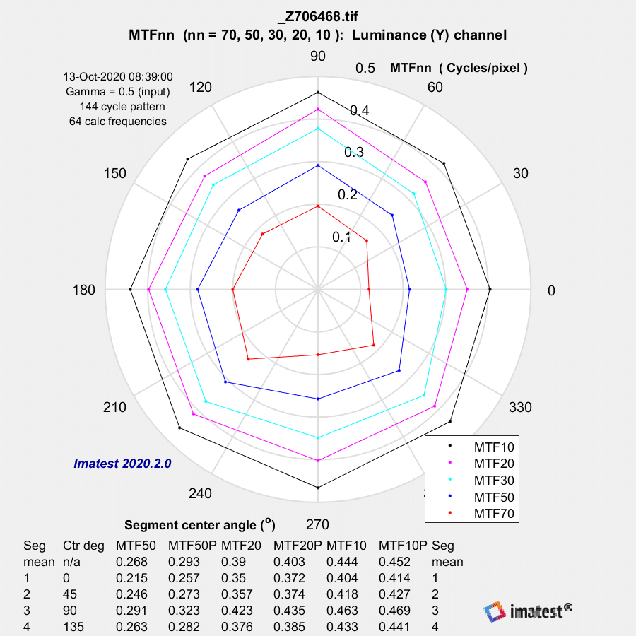
Here it is for the two lenses in the center:
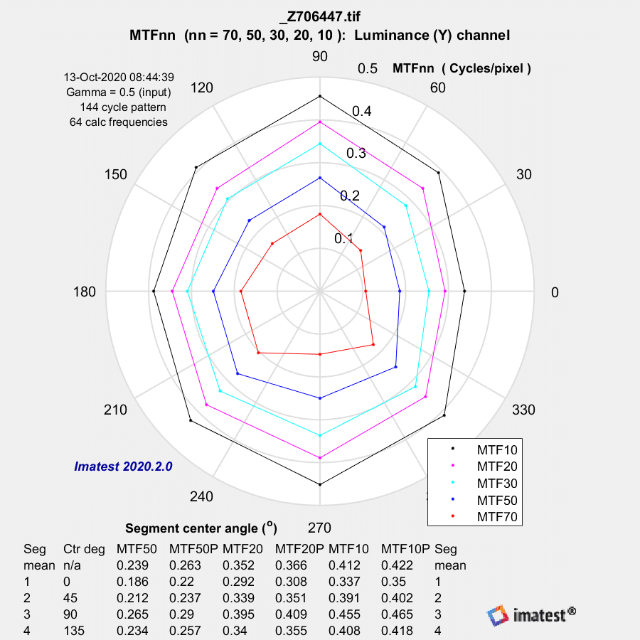
Nikon 70-200/2.8 S at 200 mm, center


Nikon 70-200/2.8 E at 200 mm, center

Those look similar.

In the corner:

Nikon 70-200/2.8 S at 200 mm, corner


Nikon 70-200/2.8 E at 200 mm, corner

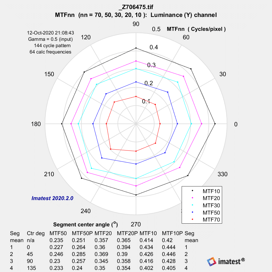
The differences are again not striking, with the E lens more symmetric.

Now for the novel approach. In this year’s version of their analysis program, Imatest has introduced a metric to gladden the heart of any computer scientist: the Shannon capacity. Here’s one of the plots associated with that metric.


Nikon 70-200/2.8 S at 200 mm, center


Nikon 70-200/2.8 E at 200 mm, center

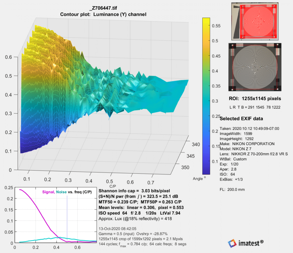
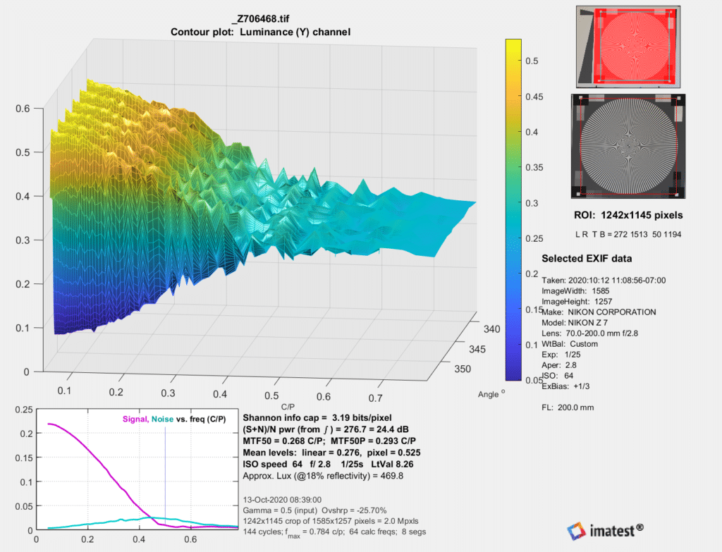
The information capacity of the S image is 3.03 bits/pixel, and that of the E image is slightly higher at 3.10 bits/pixel.

In the corner:

Nikon 70-200/2.8 E at 200 mm, corner


Nikon 70-200/2.8 E at 200 mm, corner

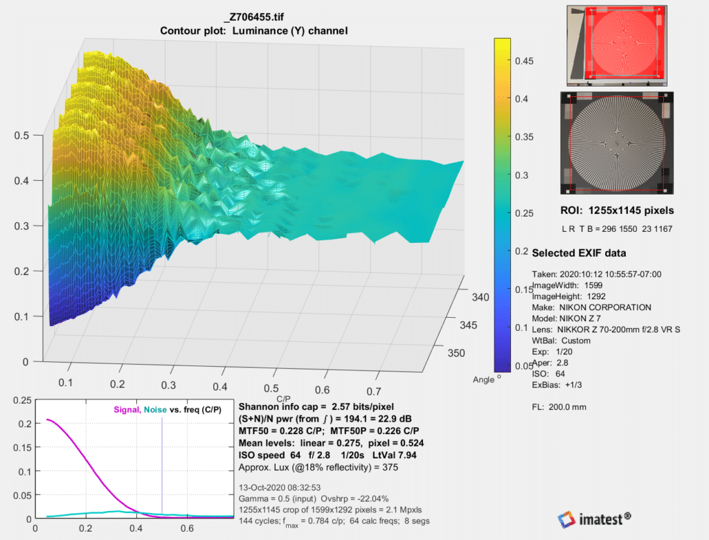
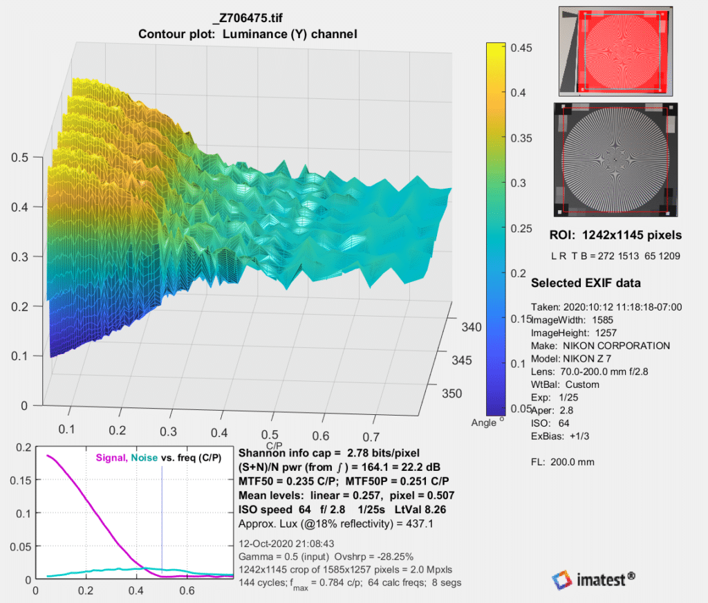
The information capacity of the S image is 2.57 bits/pixel, and that of the E image is slightly higher at 2.78 bits/pixel. Both are lower than the center images, which agrees with my visual impression.

It’s going to take some time to see how the Shannon capacity squares with image sharpness in general, but it is an interesting new metric.

Nikon Z6/7

← 70-200/2.8 E vs S at 200mm, quantitative Sony 135 STF on GFX-50R, sharpness →

Comments

  1. Ilya Zakharevich says

    October 16, 2020 at 11:18 pm

    A lot of thanks (again!) for your posts. A couple of comments for the Shannon part:
     • I analyzed how Imatest converts ITS raw data (for dynamic range reports) to what it reports to the user. Their math is COMPLETELY wrong! (It seems that the code was written a decade ago, — and it has a good chance to work with 10-years old cameras! However, the assumptions they built in are majorly broken with the technology of today.) So one should be kinda careful with what they claim. (Of course, the situation may have improved, and their new code may be better.)
     • It seems that the Shannon metric is not normalized for exposure. (This is correct — formally.) And your exposure is very different. Moreover, T-numbers may be quite different. So it may be that the reported Shannon metric is not reporting what you think it is reporting… (Cannot understand their notations, so cannot comment more.)

    Reply
    • JimK says

      October 17, 2020 at 7:53 am

      I’ve never used Imatests DR reports. Their slanted edge numbers are pretty close to MFT Mapper and my results using the Burns algorithm. I just started using the Siemens Star, and it more or less agrees with the slanted edge testing. Nice catch on the lack of normalization in the Shannon metric. Given the amount of light falloff, I guess that would invalidate center/corner comparisons, huh?

      Reply
      • Ilya Zakharevich says

        October 18, 2020 at 6:34 pm

        1st: I wrote “your exposure is very different” when I meant “your exposure is very different BETWEEN LENSES”. Sorry!

        2nd: I did not even notice that you have center/corner comparisons! And: if you ARE interested in Shannon capacity at center/corner, then these comparisons WOULD make sense ;-] — but I doubt anyone would be so crazy. If you are not interested EXACTLY in this metric — then it seems pretty useless in any OTHER situation. (Kind of black/white without any gray scale in between…)

        3rd: if you know what Imatest does with the slanted edges: what are red/green/blue curves on their graphs? Color channels vs. Y-channel?

        4th: when I wrote my own slanted-edge evaluator, I saw A LOT of forks which would RADICALLY change the results. Are you processing RAW or de-Bayered picture? Is a pixel going to be represented as a δ-function, or a square? (Or, with monitors, as a 1×3 rectangle; or, with paper print, upscaled with an arbitrarily curve…) (This is what I remember how…)

        So I cannot take your “numbers are pretty close” without a certain grain of salt…

        Reply
        • JimK says

          October 19, 2020 at 8:54 am

          Are you processing RAW or de-Bayered picture?

          Demosaiced by Lr.

          Pixels are not little squares: http://alvyray.com/Memos/CG/Microsoft/6_pixel.pdf

          Reply

Leave a Reply Cancel reply

Your email address will not be published. Required fields are marked *

May 2025
S M T W T F S
 123
45678910
11121314151617
18192021222324
25262728293031
« Apr    

Articles

  • About
    • Patents and papers about color
    • Who am I?
  • How to…
    • Backing up photographic images
    • How to change email providers
    • How to shoot slanted edge images for me
  • Lens screening testing
    • Equipment and Software
    • Examples
      • Bad and OK 200-600 at 600
      • Excellent 180-400 zoom
      • Fair 14-30mm zoom
      • Good 100-200 mm MF zoom
      • Good 100-400 zoom
      • Good 100mm lens on P1 P45+
      • Good 120mm MF lens
      • Good 18mm FF lens
      • Good 24-105 mm FF lens
      • Good 24-70 FF zoom
      • Good 35 mm FF lens
      • Good 35-70 MF lens
      • Good 60 mm lens on IQ3-100
      • Good 63 mm MF lens
      • Good 65 mm FF lens
      • Good 85 mm FF lens
      • Good and bad 25mm FF lenses
      • Good zoom at 24 mm
      • Marginal 18mm lens
      • Marginal 35mm FF lens
      • Mildly problematic 55 mm FF lens
      • OK 16-35mm zoom
      • OK 60mm lens on P1 P45+
      • OK Sony 600mm f/4
      • Pretty good 16-35 FF zoom
      • Pretty good 90mm FF lens
      • Problematic 400 mm FF lens
      • Tilted 20 mm f/1.8 FF lens
      • Tilted 30 mm MF lens
      • Tilted 50 mm FF lens
      • Two 15mm FF lenses
    • Found a problem – now what?
    • Goals for this test
    • Minimum target distances
      • MFT
      • APS-C
      • Full frame
      • Small medium format
    • Printable Siemens Star targets
    • Target size on sensor
      • MFT
      • APS-C
      • Full frame
      • Small medium format
    • Test instructions — postproduction
    • Test instructions — reading the images
    • Test instructions – capture
    • Theory of the test
    • What’s wrong with conventional lens screening?
  • Previsualization heresy
  • Privacy Policy
  • Recommended photographic web sites
  • Using in-camera histograms for ETTR
    • Acknowledgments
    • Why ETTR?
    • Normal in-camera histograms
    • Image processing for in-camera histograms
    • Making the in-camera histogram closely represent the raw histogram
    • Shortcuts to UniWB
    • Preparing for monitor-based UniWB
    • A one-step UniWB procedure
    • The math behind the one-step method
    • Iteration using Newton’s Method

Category List

Recent Comments

  • JimK on Goldilocks and the three flashes
  • DC Wedding Photographer on Goldilocks and the three flashes
  • Wedding Photographer in DC on The 16-Bit Fallacy: Why More Isn’t Always Better in Medium Format Cameras
  • JimK on Fujifilm GFX 100S II precision
  • Renjie Zhu on Fujifilm GFX 100S II precision
  • JimK on Fuji 20-35/4 landscape field curvature at 23mm vs 23/4 GF
  • Ivo de Man on Fuji 20-35/4 landscape field curvature at 23mm vs 23/4 GF
  • JimK on Fuji 20-35/4 landscape field curvature at 23mm vs 23/4 GF
  • JimK on Fuji 20-35/4 landscape field curvature at 23mm vs 23/4 GF
  • Ivo de Man on Fuji 20-35/4 landscape field curvature at 23mm vs 23/4 GF

Archives

Copyright © 2025 · Daily Dish Pro On Genesis Framework · WordPress · Log in

Unless otherwise noted, all images copyright Jim Kasson.