This is a continuation of a report on new ways to look at depth of field. The series starts here:
When I first started my investigations into depth of field management, I was driven by two very separate things that ganged up to point me in that direction.
The first was the work I did measuring longitudinal chromatic aberration (LoCA) and focus shift. My approach to that work was to mount the camera—and in some cases the razor blade target—on a motorized rail controlled by a computer. A byproduct of tests using that set up was a very accurate look at the way that sharpness, measured in terms of MTF50, varied with subject distance. At apertures close to the optimum for the lens involved if the margins of acceptable depth of field were anywhere near what the lens was capable of, the depth of field was pathetically low. I had been used to derating the marked DOF ticks on lenses by three stops, but my measurements indicated that even this wasn’t enough for critical work. That provided motivation for me to do some further study.
While I was thinking about that, I got involved in a discussion about object-field DOF management methods in the a7x forum on DPR. I had some concerns about how some of the tenets of that approach fared under conditions where there were appreciable contributions to loss of sharpness from lens aberration, diffraction, and sampling with apertures larger than the infinitesimally small points assumed by sampling theory.
It seemed that a way to get at both those things was to do simulation studies. I happened to have a camera simulator that modeled read and shot noise, diffraction, a crude lens aberration model, a Bayer CFA, and arbitrary (assumed square) fill factors. It didn’t handle defocusing, so I modified it to do so, simply adding another convolution with a pillbox kernel to model the defocusing. Alan, Severain, AiryDiscus and others have demonstrated that that’s not an accurate way to model defocusing, but let’s set that aside for the moment. The model produced spatial frequency response (SFR) curves using the slanted edge method, and I reported on MTF50 primarily.
That model ran very slowly, taking a few hours to produce each set of results. Jack Hogan produced a model that was simpler than mine, leaving out the CFA, using a monochromatic source, and making more assumptions about various kinds of blur, but the results were close enough for what I was trying to get at. Jack’s model had one huge advantage over mine: instead of running in a few hours, it never took more than a second.
Jack’s code used a different lens model than mine. His simulated lens was better than a real Zeiss Opus 85/1.4 at the wider apertures. Mine was worse. Both produced roughly similar results from f/8 to f/22.
I switched to Jack’s model – he generously supplied me his Matlab code, which I modified and extended – and produced a set of results for both image-plane and object-field MTF50.
One of the things that came out of all this modeling is that, at MTF50’s that photographers consider sharp or close to that, lens aberrations and fill factor played an important role in determining sharpness; it wasn’t all diffraction and defocusing. That made me concerned that the inaccuracies in the way defocusing was modeled in both Jack’s and my simulations was making the results of questionable value. I don’t know if making the model more accurate will change the general nature of the results or not, and that makes me question how much further I should go with the present two models. I’d hate to do a lot of work and then have to do it over.
I didn’t feel confident extending either model to include a better defocusing algorithm, as I have hardly any background in optics. I do own a copy of the classic Fourier Optics, but unfortunately, having it on my bookshelf has not increased my skills. Alan Robinson volunteered to extend Jack’s algorithm to improve its accuracy under moderate defocusing.
Here’s Alan’s algorithm for MTF = x:

Where lambda is the wavelength of the light, delta Z the defocusing distance, and Fn the f-stop.
For MTF50, this simplifies to:

I implemented this in Matlab (Alan even provided the critical code), and made a constant change in the above at Alan’s suggestion. The 2.06 in the first term of the denominator became 1.9414. I also changed the constant in the equivilant last term of Jack’s denominator to 2.2.
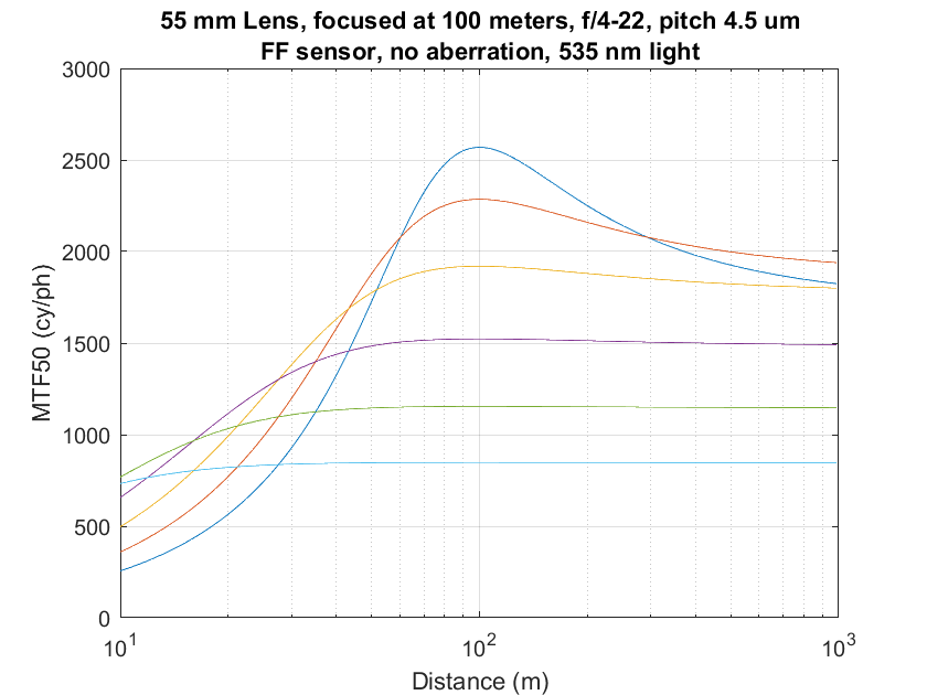
Let’s compare the results, first with no aberration and a zero fill factor (point sampling). The captions all say that the lens was focused at 100 meters. That is a lie; 10 meters is the right number.
Jack’s algorithm:

Alan’s:
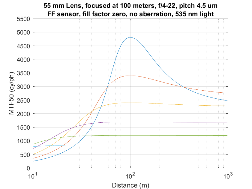
Note that the peak MTF50s are well above the Nyquist frequency for the 42MP camera that is modeled.
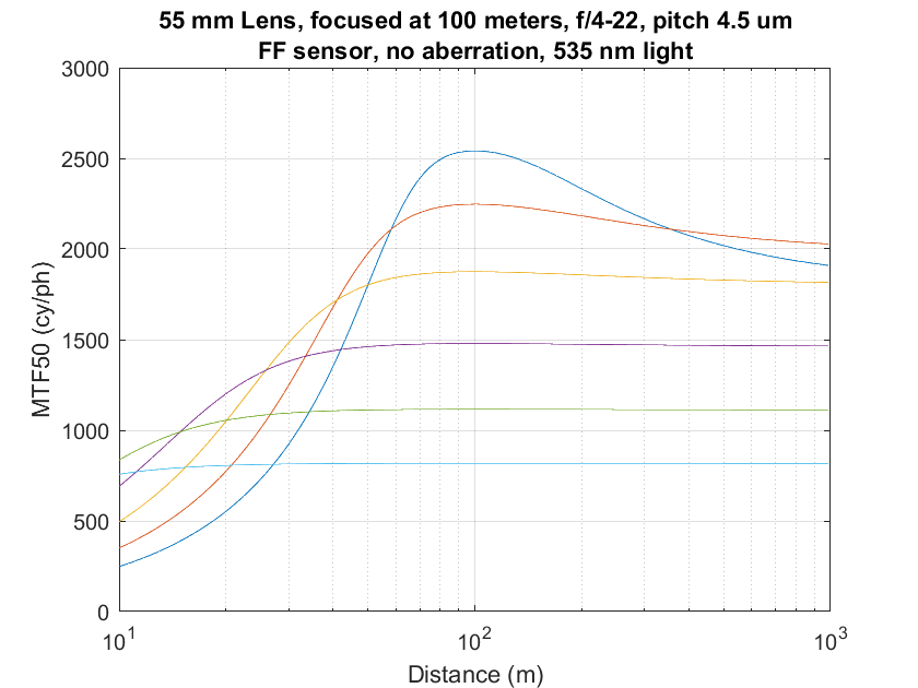
Changing the fill factor to 100% gives us a more realistic case.
Jack’s:
Alan’s:
And finally, adding our 1.4 micrometer (not pixel, like it says in the captions) lens aberration, which is optimistic at apertures wider than f/8 or so.
Jack’s:
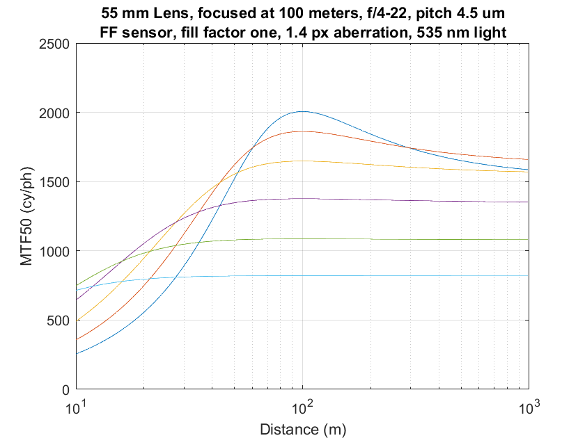
Alan’s:
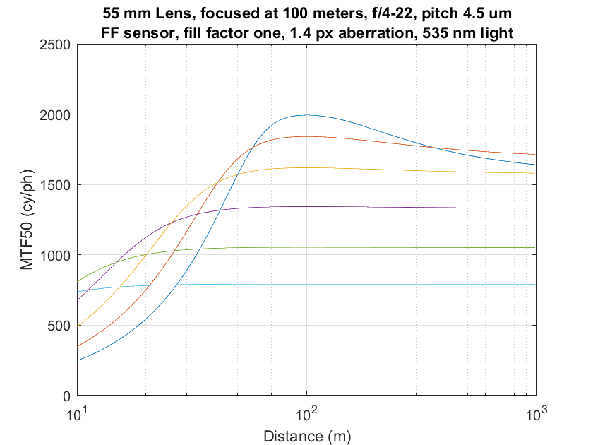
Alan’s curves are somewhat broader for wide apertures. The difference is not large.
Whew! I don’t have to go back and rework the last two weeks’ worth of posts.
[…] that I’ve got a pretty good defocusing/diffraction algorithm, it seemed like a good time to work on the rest of the lens. First, I added longitudinal chromatic […]