This is a continuation of a series of posts about blur management for landscape photography. The series starts here.
In the last post, I looked at blur circle profiles that resulted from a mixture of diffraction, pixel aperture, and defocus, and compared those profiles to the blur circle limits that I had derived from approximations. In this post, I’d like to add precision to the comparison by plotting the encircled energy as a function of distance from the center of the blur circles.
Let’s look at one such graph:
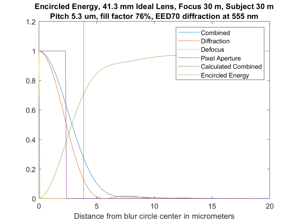
This is similar to what you saw yesterday, but I’ve only plotted the right half of the profile. We don’t lose any information by doing that, since the profiles are symmetric about their centers. The modeled aperture is f/8. What you’re looking at above is a cross-section of the blurs from each source. The yellow spike near the y-axis is the defocus blur, and in this case there’s none of that since the subject is perfectly in focus. The magenta box is the blur from the pixel aperture, which is assumed to be a pillbox with a diameter of the pixel pitch times the square root of the fill factor. The red curve is that of the diffraction. I convolved all three to get the blue curve, which is the combined effect of all three modeled blurs. And finally, the vertical line represents the limits of the blur circles that I’ve been showing you, using something called EED70 for the Airy disk diameter. The blur circle limits cross the convolved solution at about a quarter of the peak value.
There’s a new curve in the above graph. It’s green, and it’s the amount of energy that is encircled as you get further away from the center of the blur circle. It crosses the limit line at about 70%.
Here’s the same setup with the camera focused at 1000 meters:
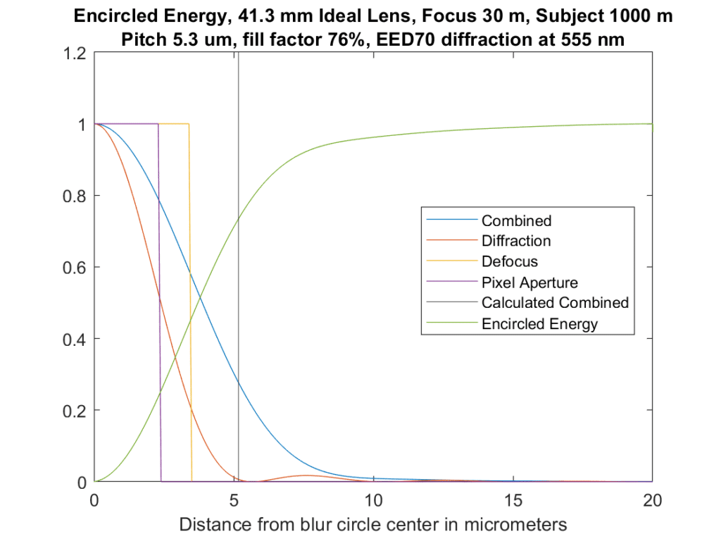
Again, the encircled energy line crosses the limit line at about 75%.
One more, with the lens focused at 8 meters, so that defocus dominates.
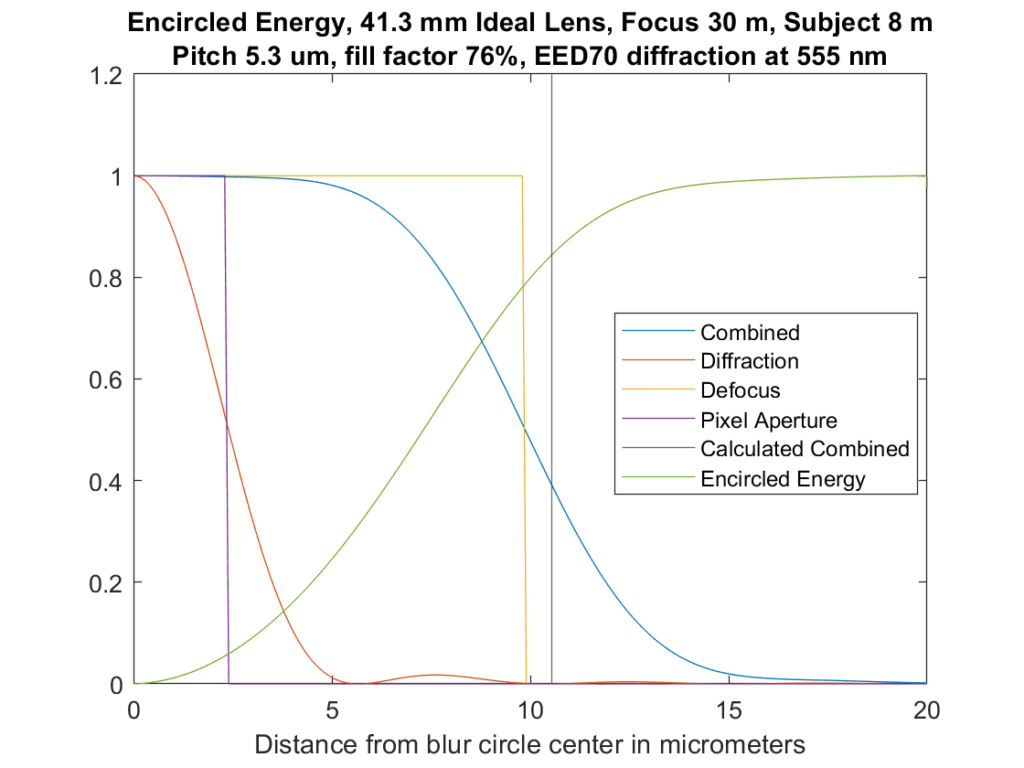
Crosses at about 85%.
What’s a good encircled energy to use for the DOF optimizer? It doesn’t make any difference to the optimal f-stops and focused distances that are found. I’m not uncomfortable with the way these graphs look. In the limit as the image becomes progressively more unfocused, the limits I’m using will converge to the normal CoC diameters.
As a check, I did a run with the focal point and the subject at 30 m (which provides no defocus blur), and the fill factor set to 0.00001% (which provides no sampling blur):
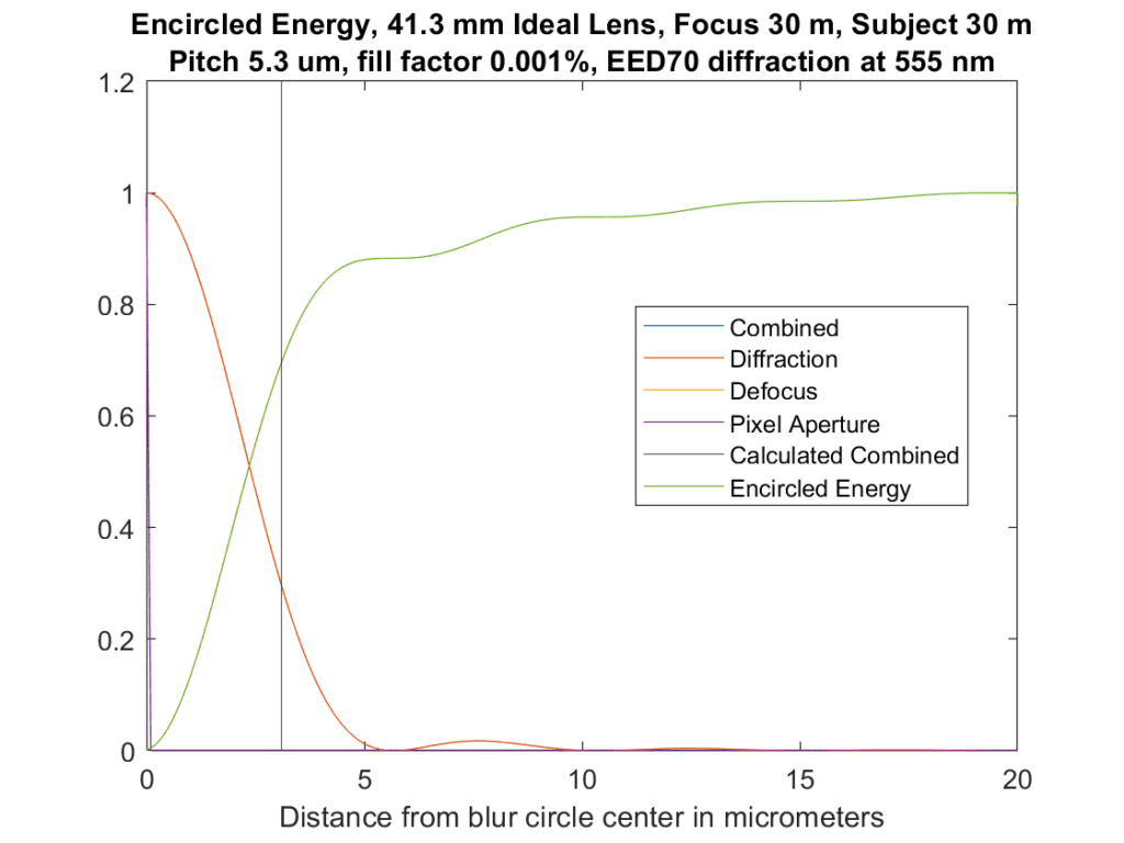
Now all we have is diffraction, and this curve is substantially the same as the one in this document.
I can make it even closer by increasing the range of distances, but that’s good enough.
How do you calculate EE? I’ve found the naive method to be garbage unless you’re ridiculously oversampled, and Baliga and Cohn’s way is not all that reliable either, +/- 2% at best, and it “turns around” and heads for zero after a large enough radius.
I’m just progressively integrating as the radius increases.
runningSum = 1.0;
result = ones(originRow+1,1); %assigns 1 to center
for r = originRow+1:nRows
runningSum = runningSum + 2 * pi * (r – originRow) * profile(r);
result(r – originRow + 1) = runningSum;
end
I’m sampling at 100 nm spacing.
Note the earlier graphs I posted were wrong. Sorry.
Well, that’s about Q=50, which I would say is (super) ridiculously oversampled.
Are you sure the results are good? For the in-focus case, the airy radius is 5.4 microns, at which point you would expect 83.8% encircled energy from just diffraction. The blur is larger with other factors, so we should expect less EE, maybe something like 60% even. Your plot looks to be around 90% or so, which would be the case for the second zero of the airy pattern (90.9%, anyway).
I can send you the analytic form for the EE of the airy pattern if you want to do some investigation of (technique) vs truth. I suspect you have a domain-not-large-enough problem.
I’d be happy to see the analytic form. I see what you mean about the domain size. I’ll look at that in the morning.
Thanks.
Sure — the equation is 1 – J0^2(r) – J1^2(r), where J0 and J1 are bessel functions.
I emailed you a plot I made with prysm – it has a curve for just the airy disk, numerically derived using Baliga and Cohn’s method, and for the AD convolved with a pixel aperture equal to 5.3*.76 um in diameter, calculated the same way. You should expect wiggles in the EE, related to the zeros of the airy disk. It seems the pixel aperture serves to wash those away, which makes intuitive sense since the rings will blur into the ‘valleys’ so to speak.
I found an error in the EE calculation. Now it’s:
runningSum = 0.0;
result = zeros(originRow+1,1);
for r = originRow:nRows
runningSum = runningSum + …
pi * ((r + 1 – originRow)^2 – (r – originRow)^2) * profile(r);
result(r – originRow + 1) = runningSum;
end
I revised the graphs and added a diffraction-only graph to the post as a check . It looks pretty much the same as the plot that I found in a set of Cal Tech lecture notes:
http://web.ipac.caltech.edu/staff/fmasci/home/astro_refs/PSFtheory.pdf
Thanks for all your help.
Even better: trapezoids instead of rectangles for the integration:
runningSum = 0.0;
result = zeros(originRow+1,1);
for r = originRow:nRows
runningSum = runningSum + …
pi * ((r + 1 – originRow)^2 – (r – originRow)^2) * …
((profile(r) + profile(min(r+1,nRows))) / 2.0);
result(r – originRow + 1) = runningSum;
end
Hi Jim,
Defocus disk diameter = 8NW20. Based on your 1000m plot above, at f/8 that would mean that W20 is 16/64=0.25um about 1/2 lambda. Take a look at the 1/2 lambda PSF in Figure 2 below: not quite a top hat
https://www.strollswithmydog.com/simple-model-for-sharpness-in-digital-cameras-spherical-aberration/
8 fno squared, not 8 fno. The correct notation is W020, not W20.
No, the diameter of the geometrical defocus disk is 8N*W20, do your homework before speaking out of your derriere.
As for W20 vs W020 see H.H.Hopkins – and whatever.
Well, it LOOKS so much wrong that I do not even know where to start…
First of all, are you assuming a coherent source, or a non-coherent one? Are you assuming a “point” source, or a “linear” source? It looks like you are taking different assumption in different sections of your calculations…
For example, for a point source defocus would give √(r²-x²) instead of a pillbox…
> “I convolved all three to get the blue curve, which is the combined effect of all three modeled blurs.”
Nope, taking convolution is not a correct way to combine the defects. (I’m not fully woken — maybe it IS correct for a non-coherent source? Definitely not for a coherent one…)
Incoherent source. I don’t generally photograph coherent sources.
How do you know? Coherence has a measure: coherence length. For example, look at two possible paths through a defocused lens. Say that the optical paths differ by 1µm. Would these rays create an interference pattern, or would they de-phase enough to “not interfere”?
Myself, I’m very fuzzy about the order of magnitude of coherence length from natural sources. I could not find a source I can trust…
These are for point spread functions.
Then, as I said, the “base curve” for defocus is wrong. (It cannot be the same as for the square sensel, right?)
It is approximately the same, since there is falloff on microlens coverage in the corners.
Well, then *both* need to be fixed…
Please construct a model the way you think is right, test it, post the results, and then come back here and post a link to that post in these comments.
Got your point! Sorry, Jim, if this came up as patronizing!
Let me retry: ”**In a perfect world,** *both* would need to be fixed…” 😉
======================
(BTW: I did. Many years ago. But you have the same ability to google for it as I. — I do not remember were/how I published it. Probably on Google Groups???)
And: my model ALSO did not take into account finiteness of the length of coherence (even NOW, after a decade or two, I do not know how to do it!). And, definitely — and obviously, it was not as nicely written as what you do!
Finally: this looks just a proper place to remind how much I appreciate all that you do! (THIS is the main reason for my : when I see that tiny changes may improve it, I want to point it out. The purpose is absolutely not to annoy you! Sorry again!)
Oups, it looks like your posting software does not allow ⟨less-than⟩ and ⟨greater-than⟩ marks! The unclear place in the preceding post should look like:
“THIS is the main reason for my ⟨pedantic mode/⟩: when I …”
It allows html. That’s a side effect.