Yesterday I wrote a post aimed at discovering the relationship between dither and quantizing precision when resolving detail was the main criterion. The conclusion was that, just as for the avoidance of posterization (see here, here, and here), half a least-significant bit (LSB) was enough noise for most purposes. For critical judgements, it looked like 0,7 bits was slightly better.
For that test, I used about the most simpleminded demosaicing algorithm, bilinear interpolation. Today, I’m going to present results using a more sophisticated algorithm, adaptive homogeneity-directed demosaicing (AHD).
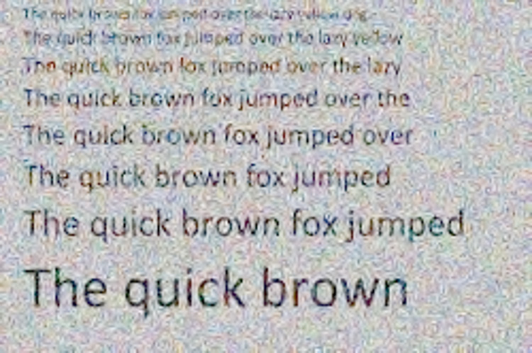
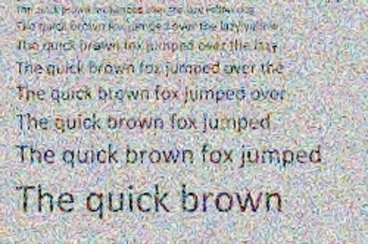
Here’s the test image:

It’s go no tones near white or black, so over and undershoot won’t be a problem. I reprogrammed my camera simulator to ignore photon noise, apply read noise only after the amplifier with rms value equal to a specified number of LSBs of the ADC. I ran the ADC at 3, 4, and 5 bits of precision. This gives the same effect as large Exposure pushes on underexposed images with cameras of greater precision.
Other model details:
- f/2 diffraction-limited lens
- 450, 550, and 650 nm light
- 4.88 um pixel pitch
- Adobe RGB GBRG CFA (I had to change the Bayer pattern to work with the AHD Matlab code I’m using)
All images are presented here enlarged to triple the camera resolution.
Here’s a set with noise equal to half an LSB of the 3 bit converter, a full LSB for the 4 bit converter, and 2 LSBs for the 5 bit converter. Thus the noise voltage remains the same if the full scale voltage remains the same, regardless of the precision of the ADC.
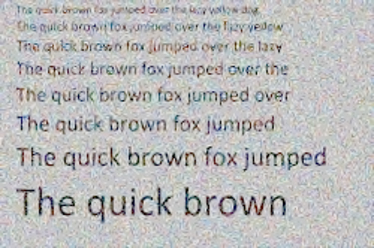
I think the differences are even smaller than with bilinear interpolation, but you can judge for yourself.
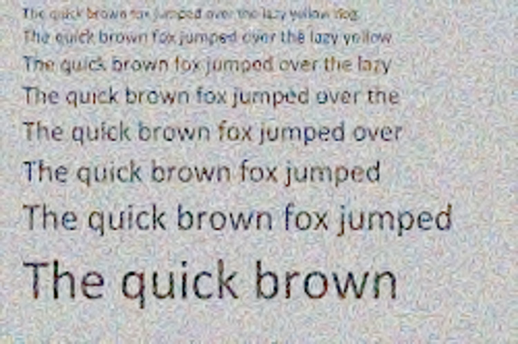
Increasing the dither a bit, to 0.7 LSB of the 3 bit converter, 1.4 LSB for the 4 bit converter, and 2.8 LSBs for the 5 bit converter:
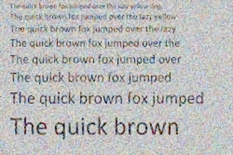
As before, I’d call the differences that don’t relate to the character of the noise itself inconsequential. The noise is indeed more smoothly rendered with higher precision; no surprise there.
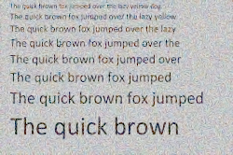
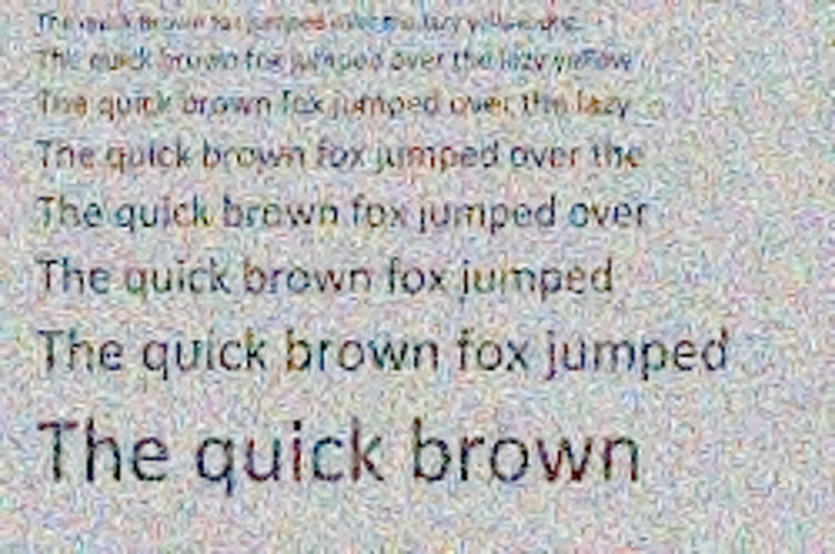
Increasing the dither to 1 LSB of the 3 bit converter, 2 LSB for the 4 bit converter, and 4 LSBs for the 5 bit converter (a somewhat smaller step than yesterday’s last set of images):
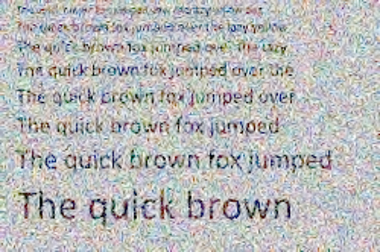
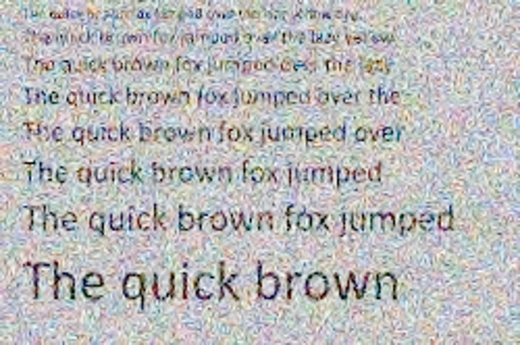
What do you all think?
Jim, I’m not sure how this translates to pictures, but for audio, Gaussian distribution noise isn’t great because it doesn’t uncouple all of the error moments from the signal itself: ie. you can hear patterns in the noise modulated by the signal itself. They like to use triangular probability distribution function noise which uncouples the first and second order error moments. The idea is to uncouple (decorrelate) any relationship the noise has to the signal, so that it allows the ear to pick out signal below the noise given sufficient listening (integration or averaging) time.
As it turns out, I’m well aware of that:
http://www.google.com/patents/US4187466
However, the objective here is to find out how much read noise it will take to properly dither the signal in a gamera, and read noise is usually close to Gaussian.
Jim
Hmm … I’m not sure that’s the same thing since your invention uses what sounds like a rectangular PDF (“uniform probability density function”). TPDF can be synthesized by adding two RPDFs.
Anyway, a philosophical question: if a given PDF, like Gaussian, does not decouple error, would adding any amount of it be able to properly dither a signal?
That’s an angels/pinheads question for a mathematician. I can attest that it makes a tremendous improvement, so much so that precision stops mattering soon after it sinks below the level of the read noise.
Jim
Hi Jim, very interesting test. If you want to compare all demosaicing code, you can use the software RawTherapee.
I use RAW-files from dpreview: http://www.dpreview.com/reviews/fujifilm-x-pro2/7
This test-chart have in the middle three text version.
And with RawTherapee you can test all demosaicing-code (amaze, lgv, vng, dcb, immse, eahd, ahd, fast, mono and none).
I use rawtherpee to find out, which demosacing-code is the best for raw-file from each manufacturer! I found out, even between the different model from the same manufacturer, the best demosaicing-code is not always the same!
When the pixel-pitch is higher different demosaicing-code do not affect much. But, if the pixel-pitch is small, then it is required to find out the best demosaicing-code.
And least, for the newest bsi-sensor pixel-pitch the sience have to invest to find out newer algorithm for demosaicing! With newer much accurate algorithm the demosaicing would be much much better. And also the noise would be better.
I don’t know how to create something in Matlab that a commercial raw converter will recognize as a raw file. Any ideas? I’ve looked at using the Adobe DNG toolkit, but it looked really complicated for the simple thing I’m trying to do. So, for the time being, I’m stuck with demosaicing algorithms I can run in Matlab.
Jim
Jim, I haven’t tried it, but if it’s possible to read the raw cfa data in a DNG file it should be possible to write to it. Check loadImg in the last file I sent you for the simple code to read it.
Jack
First RawTherapee is not comercial, it is free (open source).
I am only project manager and has some works with programmer. I am not a programmer.
I find a good website with “newer” demosaicing-code for matlab. http://www.ok.ctrl.titech.ac.jp/res/DM/RI.html
Take a look. At the end of the page, you can see the newer algorithm!! Very interesting. And on this chart you can see, that AHD was developped on 2005! In 11 year the CMOS has evolved, and AHD is no longer appropriate……
As far as I know, the demosaicing algorithm for a Bayer sensor is not coupled to chip technology at all, except that the demosaicing must know the CFA pattern. Theere are only 4 possibilities, if we’re talking EGB patterns.
Jim
Are you using the same noise pattern for each bit depth?
It doesn’t look like it, so readability might vary randomly between runs and it’ll be hard to fairly compare the different bit depths.
No. I will look at doing that.
Jim