Does Sony raw compression damage images?

There’s a lot of Internet talk about whether the compression algorithm that Sony uses in the a7, the a7R, and several other cameras cause visible damage to the images. The furor seems to be gaining intensity rather than dying down. Because of that, I’ve decided to do something that I’ve resisted in the past, which is simulate the Sony algorithm.

I’ve written Matlab code to take real or synthetic images, capture them to a simulated sensor with programmable amounts of antialiasing, lens blur, pixel translation, and motion blur. The program then demosaics the image using bilinear interpolation. I added some processing for the Sony algorithm, notably, tone compression from 13 to 11 bits, delta modulation in groups of 16 pixels and its inverse, and tone decompression from 11 to 13 bits.

I think the code would be Too Much Information for this blog; it’s much longer than the Matlab snippets I’ve posted in the past. I will go into the compression and decompression in words, however.

The tone curve applied to the 13-bit linear data is a linear interpolation between a curve defined by these input points: 0 1000 1600 2854 4058 8602, and these output points: 0 1000 1300 1613 1763 2047.

The delta modulation extracts successive groups of 32 pixels within a single row. Because of the RGGB Bayer color filter array, that gives 16 green pixels in all rows, 16 red pixels in the odd rows, and 16 blue pixels in the even rows. Odd and even are defined assuming that the first row is row 1.

As an example, an odd row would start out RGRGRGRGRG… and an even row would begin GBGBGBGBGB…

For each group of 16 pixels, the maximum and minimum 11-bit values are found, and the indices of those values recorded as two four-bit numbers. The minimum is subtracted from the maximum to give a number that I call the span.

Then a value called the step is calculated. If the span is equal to or less than 128, the step is 1. If the span is more than 128 and equal to or less than 256, the step is 2. . If the span is more than 256 and equal to or less than 512, the step is 4. If the span is more than 512 and equal to or less than 1024, the step is 8. Otherwise the step is 16.

For each of the remaining 14 pixels, the minimum value is subtracted, and the result divided by the step size, truncated (or rounded; that’s what I did) and encoded as a 7-bit number which is stored. Thus we have 16 pixels encoded in 16 bytes (11*2 + 4*2 + 7*14, or 128 bits). The algorithm proceeds across all the columns in a row, then moves to the next row down, does it again, until it runs out of rows. That’s what’s in the raw file.

The process is reversed in the raw converter. The original 11-tone compressed values are recovered by inverting the delta modulation algorithm – I leave that as an exercise for the interested student – and the tone curve is removed by a linear interpolation between a curve defined by these input points: 0 : 0 1000 1300 1613 1763 2047, and these output points: 0 1000 1600 2854 4058 8602.

For the above algorithm, I am indebted to Alex Tutubalin (warning: Alex’s web page is in Russian) and Lloyd Chambers. Any errors, however, are my responsibility. Please let me know if you see anything wrong.

In the actual camera, there’s some messing around with the black point. I did not simulate that.

As you can see, the tone curve leaves out progressively more possible values as the pixel gets brighter. This mimics the 1/3 power law that defines human luminance response. The questions are, are there a sufficient quantity of buckets at all parts of the tone curve, and after an image is manipulated in editing, do artifacts that were formerly invisible become intrusive?

The other possible place where visible errors could be introduced is in the delta modulation/demodulation. If the maximum and minimum values in a 16-bit row chunk are further apart than 128, information will be lost. Is that a source of visible errors?

And the last question: even if the above errors could be visible with synthetic images, are they swamped out by photon noise in real camera images?

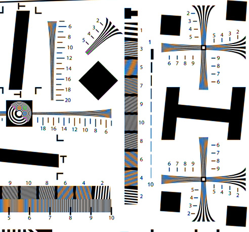
I decided to make things as hard on the compression algorithm as I could. I took and entirely synthetic image with a lot of big jumps, the ISO 12233 target, encoded it at 960×640 pixels with the simulated camera, and compared the results with and without the Sony raw compression/decompression.

Here’s a crop from the uncompressed image:

I’d show you the compressed/uncompressed version, but it look identical. Here’s the difference between that image and the uncompressed image, with 10 stops (!) of Exposure gain applied in Photoshop:

The difference between the two images was computed in Photoshop using the Difference layer blending mode, which operates in the working color space. These images were in Photoshop in Adobe RGB, which has a gamma of 2.2, and will thus tend to suppress highlight differences as compared to a linear representation. This is appropriate for visual comparisons, as the eye works in much the same way but with a gamma of three.

On this one image, there isn’t much to worry about. However, other images may prove more difficult. I welcome reader submission of candidates. I’ll also be doing more work myself, including more testing of the simulator than the initial work I did this morning.