• site home
  • blog home
  • galleries
  • contact
  • underwater
  • the bleeding edge

the last word

Photography meets digital computer technology. Photography wins -- most of the time.

You are here: Home / The Last Word / For photo-nerds only — LSF

For photo-nerds only — LSF

February 16, 2016 JimK 4 Comments

This is a continuation of a test of the following lenses on the Sony a7RII:

  • Zeiss 85mm f/1.8 Batis.
  •  Zeiss 85mm f/1.4 Otus.
  • Leica 90mm f/2 Apo Summicron-M ASPH.
  • AF-S Nikkor 85mm f/1.4 G.
  • Sony 90mm f/2.8 FE Macro.

The test starts here.

A reader thought that point spread functions (PSFs) might be better for analyzing chromatic aberration. Imatest can’t do those, but it can do the one-dimensional cousin, the line spread function (LSF).

I gave it a try. Batis wide open, on-axis vertical edge:

Batis 18 LSF

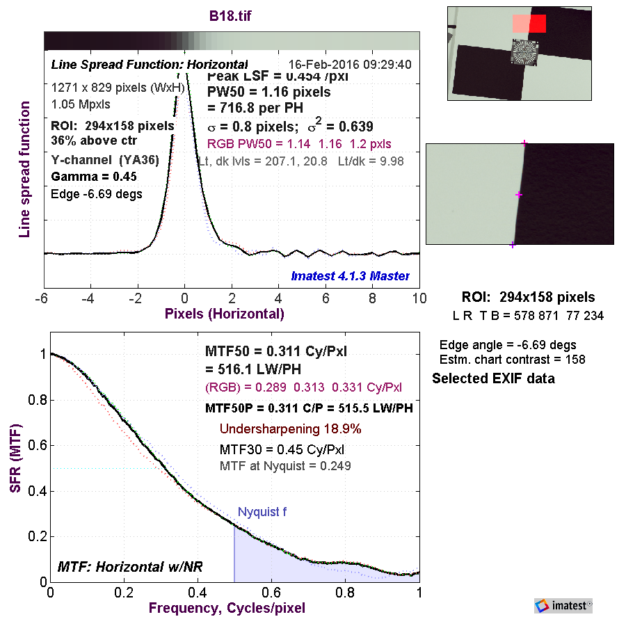
Nikon wide open, same edge:

Nikon 14 LSF

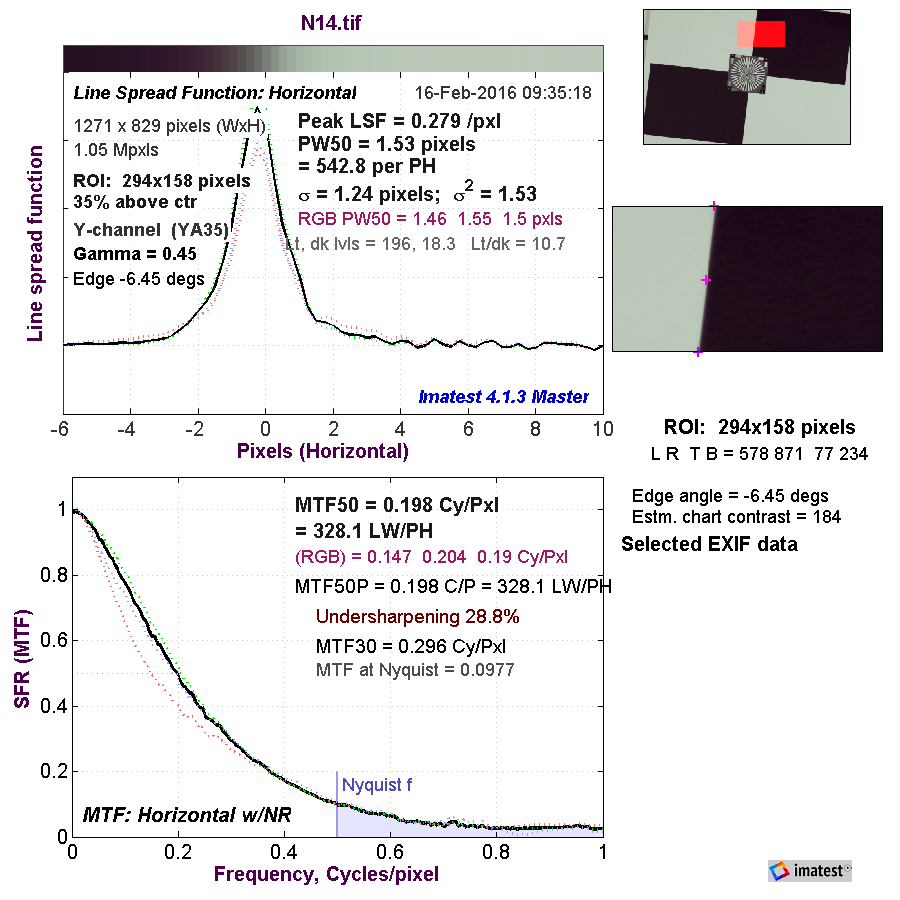
The first thing that’s wrong is that Imatest writes text over the part of the graph you really want to see. The second thing is that I don’t think this is as intuitive as the other CA plots we’ve been looking at.

[Addendum follows}

Jack Hogan sent me a LSF that he did with MTF Mapper that doesn’t have text all over it.

Jack Hogan LSF

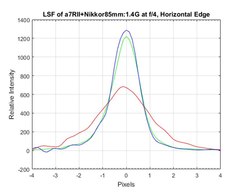
I can see that it’s telling me that the blue is the sharpest, followed by the green, with the red far in arrears. I can’t tell what it’s saying about CA though, except for the slight shift to the left for the red layer.  The location of the peaks may be a good indication of how much shift there is with wavelength, but I’m at a loss to look at a curve like this and say how visible the CA is. Anybody want to help out?

The Last Word

← Another medium tele test — more on-axis color fringing Lens quality control →

Comments

  1. CarVac says

    February 16, 2016 at 11:03 am

    Indeed I really don’t like the presentation here. You could simplify it by simply rendering it as an image with the actual brightness values, rather than a graph.

    Reply
  2. Erik Kaffehr says

    February 16, 2016 at 9:59 pm

    Hi,

    I think Jack’s plot is illustrative, one possible interpretation may be that red is spread over a larger area than blue and green. That may be caused by red (long wave lengths) having different focus than short wave lengths.

    I feel that in engineering a good graph can say more than a thousand pictures. NASA of course doesn’t think so, they present a lot of lovely images of planets detected by Kepler instead of the curves.

    🙂 Erik 🙂

    Reply
  3. CarVac says

    February 17, 2016 at 10:08 am

    Based on the addendum, you should make a 2d graph of the brightness distributions of the line spread function as you focus bracket. That’ll show when you have green OOF on one side and red/blue OOF more on the other side.

    Reply
    • Jim says

      February 17, 2016 at 10:22 am

      That sounds like a good way to get a more direct handle on LoCA.

      Reply

Leave a Reply Cancel reply

Your email address will not be published. Required fields are marked *

May 2025
S M T W T F S
 123
45678910
11121314151617
18192021222324
25262728293031
« Apr    

Articles

  • About
    • Patents and papers about color
    • Who am I?
  • How to…
    • Backing up photographic images
    • How to change email providers
    • How to shoot slanted edge images for me
  • Lens screening testing
    • Equipment and Software
    • Examples
      • Bad and OK 200-600 at 600
      • Excellent 180-400 zoom
      • Fair 14-30mm zoom
      • Good 100-200 mm MF zoom
      • Good 100-400 zoom
      • Good 100mm lens on P1 P45+
      • Good 120mm MF lens
      • Good 18mm FF lens
      • Good 24-105 mm FF lens
      • Good 24-70 FF zoom
      • Good 35 mm FF lens
      • Good 35-70 MF lens
      • Good 60 mm lens on IQ3-100
      • Good 63 mm MF lens
      • Good 65 mm FF lens
      • Good 85 mm FF lens
      • Good and bad 25mm FF lenses
      • Good zoom at 24 mm
      • Marginal 18mm lens
      • Marginal 35mm FF lens
      • Mildly problematic 55 mm FF lens
      • OK 16-35mm zoom
      • OK 60mm lens on P1 P45+
      • OK Sony 600mm f/4
      • Pretty good 16-35 FF zoom
      • Pretty good 90mm FF lens
      • Problematic 400 mm FF lens
      • Tilted 20 mm f/1.8 FF lens
      • Tilted 30 mm MF lens
      • Tilted 50 mm FF lens
      • Two 15mm FF lenses
    • Found a problem – now what?
    • Goals for this test
    • Minimum target distances
      • MFT
      • APS-C
      • Full frame
      • Small medium format
    • Printable Siemens Star targets
    • Target size on sensor
      • MFT
      • APS-C
      • Full frame
      • Small medium format
    • Test instructions — postproduction
    • Test instructions — reading the images
    • Test instructions – capture
    • Theory of the test
    • What’s wrong with conventional lens screening?
  • Previsualization heresy
  • Privacy Policy
  • Recommended photographic web sites
  • Using in-camera histograms for ETTR
    • Acknowledgments
    • Why ETTR?
    • Normal in-camera histograms
    • Image processing for in-camera histograms
    • Making the in-camera histogram closely represent the raw histogram
    • Shortcuts to UniWB
    • Preparing for monitor-based UniWB
    • A one-step UniWB procedure
    • The math behind the one-step method
    • Iteration using Newton’s Method

Category List

Recent Comments

  • JimK on Goldilocks and the three flashes
  • DC Wedding Photographer on Goldilocks and the three flashes
  • Wedding Photographer in DC on The 16-Bit Fallacy: Why More Isn’t Always Better in Medium Format Cameras
  • JimK on Fujifilm GFX 100S II precision
  • Renjie Zhu on Fujifilm GFX 100S II precision
  • JimK on Fuji 20-35/4 landscape field curvature at 23mm vs 23/4 GF
  • Ivo de Man on Fuji 20-35/4 landscape field curvature at 23mm vs 23/4 GF
  • JimK on Fuji 20-35/4 landscape field curvature at 23mm vs 23/4 GF
  • JimK on Fuji 20-35/4 landscape field curvature at 23mm vs 23/4 GF
  • Ivo de Man on Fuji 20-35/4 landscape field curvature at 23mm vs 23/4 GF

Archives

Copyright © 2025 · Daily Dish Pro On Genesis Framework · WordPress · Log in

Unless otherwise noted, all images copyright Jim Kasson.