Fundamental camera noise parameters

I’ve been posting shadow noise curves for a while. Here’s an example:

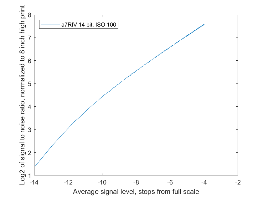
There’s a lot to unpack, but for now, just concentrate on the following:

• The curves are normalized to standard sized prints; differences in camera resolution are normalized out
• Higher y-axis values are better — they mean less visible noise
• The further to the left, the deeper the shadows
• Zero on the right is the brightest exposure the camera can handle; this graphs doesn’t go that far
• Middle gray is about -3.5 stops on the horizontal axis; we’re looking at the darker tones in the image here.
• Minimally acceptable SNR for small prints (about 8 inches high)  is marked by the horizontal line that intersects the y-axis at 3.3.

Now I’m going to walk you through how I got to that curve, with emphasis on how the fundamental characteristics of the camera determine them.

Let’s look at another set of curves relating noise and average brightness. This set has less processing, and I’ve plotted a curve for each of three different cameras.

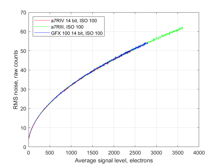
Digital camera are basically electron counters. Incoming light knocks loose electrons, which are then stored on a capacitor, and read out to end the exposure, of after the exposure has been ended mechanically. The more electrons, the brighter the pixel. But there’s noise associated with the counting. The most important components of that noise are read noise, and photon, or shot, noise.

The read noise is more or less constant with brightness. You can get a pretty good handle on it by looking at photographs of the back of the body cap or lens cap. It varies with ISO setting, shutter speed, and temperature. It can also change with camera shutter mode.

The photon noise is an inevitable effect of counting photons or electrons. It has Poisson statistics, which are similar to Gaussian ones for average signal levels of more than a handful of photons. The standard deviation of the photon noise is the square root of the mean level.

There is a third kind of noise in the curves above. It’s called pixel response non uniformity, or PRNU. In today’s cameras, it’s usually unimportant. For completeness, I included it in the model used to generate the curves above, but you can’t see its effect on them.

It turns out that the mathematics of calculating the standard deviation is identical to that for computing a common amplitude measurement, root-mean-square, or rms. If you live stateside, your wall voltage is probably about 117 volts rms.

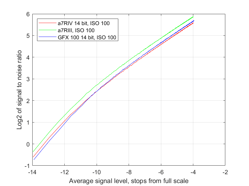
The curves above look very similar, don’t they? Part of that is that they are linear. That is a mathematically easy way to look at things, but it doesn’t correspond well to the way our vision works. For that, it is better to plot logarithmically. Here’s the same data plotted that way:

Now the upper right portion of the curves are right on top of each other, but the the lower left curves, at least in the case of the a7RIV, are different. The upper right curves are in the region where the photon noise is the main determinant of the overall noise level, and the curves are right on top of each other because the photon noise, at least looked at this way, is not affected by the sensor technology.

A more meaningful horizontal axis is the mean signal level as a fraction of full scale. the number of electrons for full scale at base ISO is determined by the full well capacity (FWC) of the sensor. Keeping the logarithmic axes, abut changing the base of the logarithm to 2 instead of 10, because photographers like to think in terms of stops, we get this:

If you are interested in noise at the pixel level, this is the set of curves to look at. But I think it is more useful to consider the noise and SNR for same-sized prints. When that normalization is applied, we get:

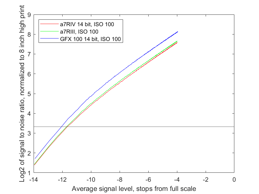
You don’t need a lot of information to generate the curves above, just the read noise at the ISO setting, the full well capacity, and the height of the image in pixels. I used the PRNU, too, but it made no noticeable difference at the scale you’re seeing here; if I’d have plotted the curves all the way up to a mean level of full scale, there might have been some visible difference. Modeled curves track measured ones extremely well.

You can tell the region where the read noise is the long pole in the tent and the one where photon noise dominates by looking at the slope of the lines in the chart above. Down to about 9 stops from full scale, photon noise dominates in the graph above. That’s the same for all three cameras. Below 12 stops down, read noise plays the larger role. In between, both contribute.

There is a possible further improvement for these charts: measure the actual sensor sensitivity, rather than trusting the camera manufacturer’s ISO settings to fairly represent sensitivity. I experimented with this, but found that the test setups were fiddly, the tests were time consuming, and there was an issue of long-term calibration. So I don’t do this, even though I have noticed variations among manufacturers, and occasionally, in different model numbers from the same manufacturer.