• site home
  • blog home
  • galleries
  • contact
  • underwater
  • the bleeding edge

the last word

Photography meets digital computer technology. Photography wins -- most of the time.

You are here: Home / The Last Word / Leica 180/3.4 Apo-Telyt-R on Sony a9: field tilt, curvature, astigmatism

Leica 180/3.4 Apo-Telyt-R on Sony a9: field tilt, curvature, astigmatism

August 15, 2017 JimK 7 Comments

This is a continuation of the development of a simple, relatively foolproof, astigmatism, field curvature, and field tilt test for lens screening. The first post is here.

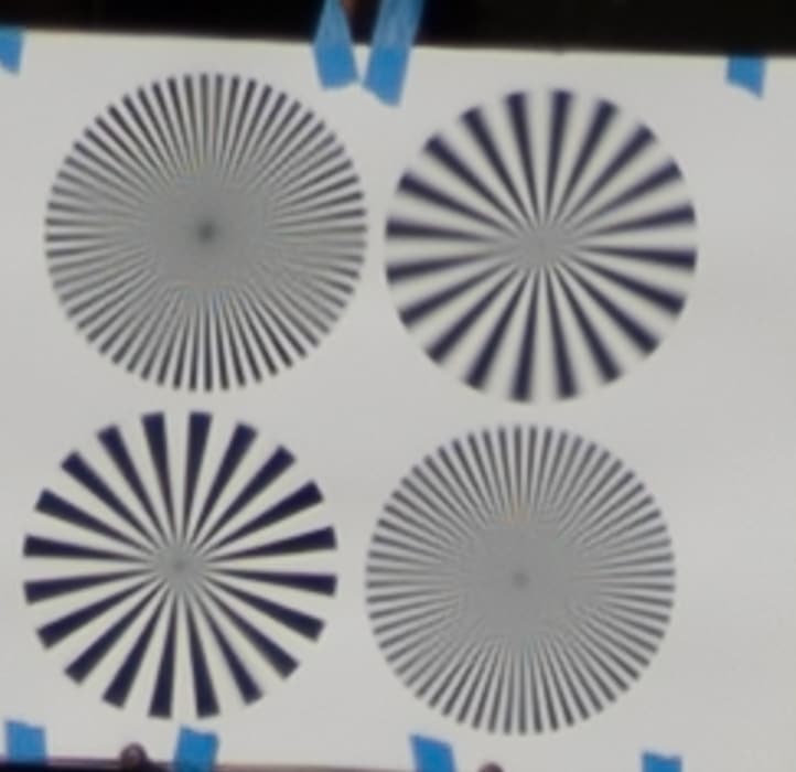
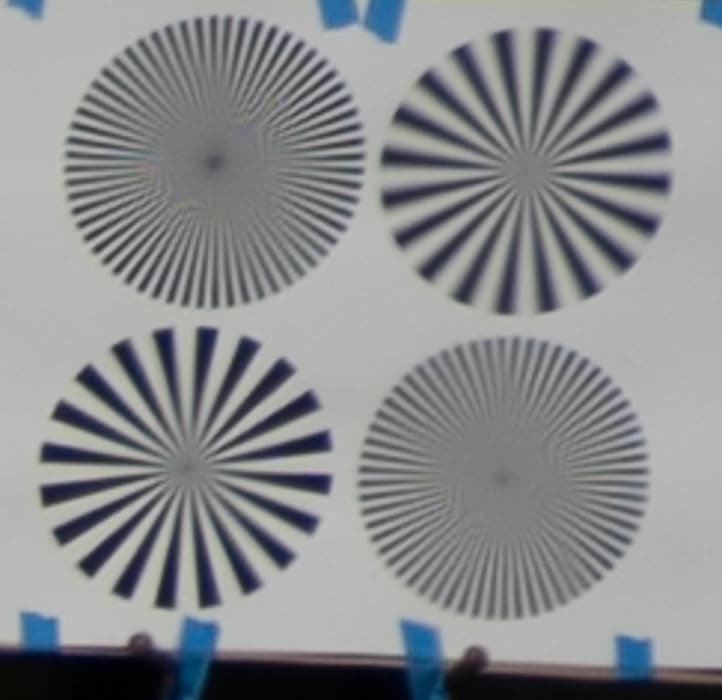
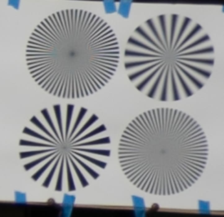
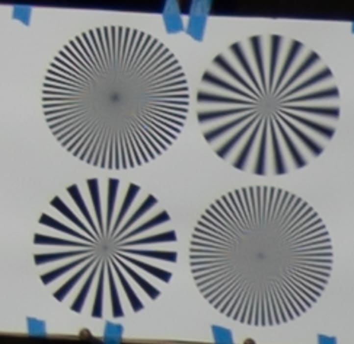
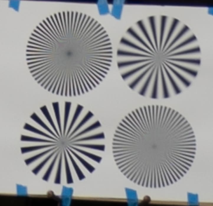
Bart van der Wolf recommended that I use a sinusoidal Siemens Star rather than the binary one. I wrote some Matlab code and made this:

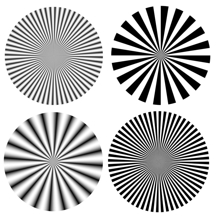
There is a fine and a coarse version of each type of star.

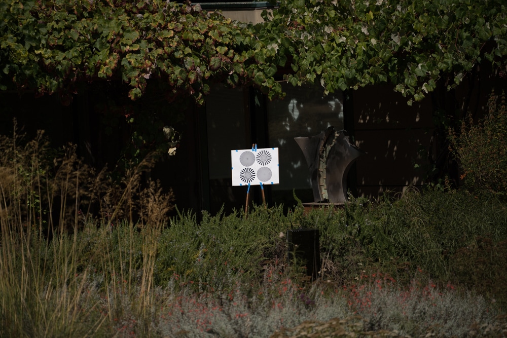
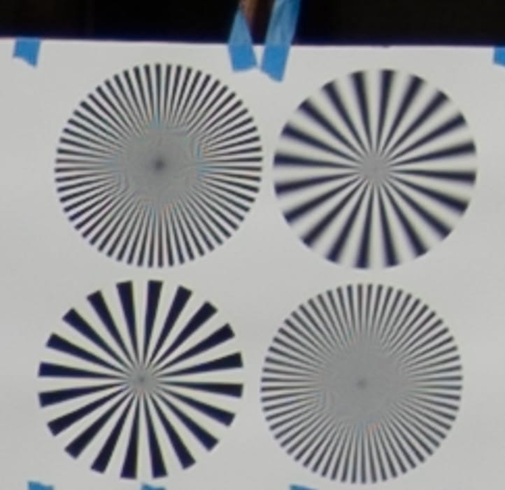
I set up with the Leica 180 mm f/3.4 Apo-Telyt on the Sony a9 at 57 meters from the target:

Here is the center:

Center

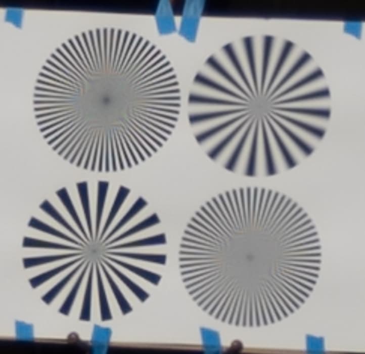
I see the target is upside down. You can see aliasing on both the fine stars. There is more on the binary one. The two coarse stars are useless at this distance.

Now we’ll go around the outside of the image clockwise, starting at the upper left corner.

Upper left

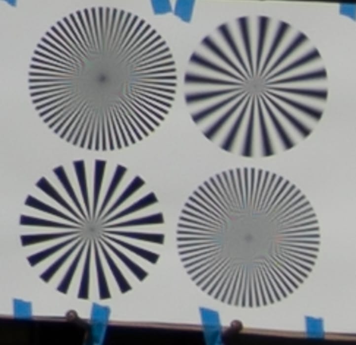
This is the sharpest image here, by a hair. I don’t think that is because the lens is sharpest off-axis. I think that a combination of slight misfocusing and field tilt makes it look that way. But I’m still learning about this test. There is a little bit of asymmetric behavior in the aliased region at ten o’clock.

Upper center

Not quite as sharp as either upper corner.


Upper right


Center Right


Lower Right

Quite harp here, too.

Lower Center


Lower Left


Center Left

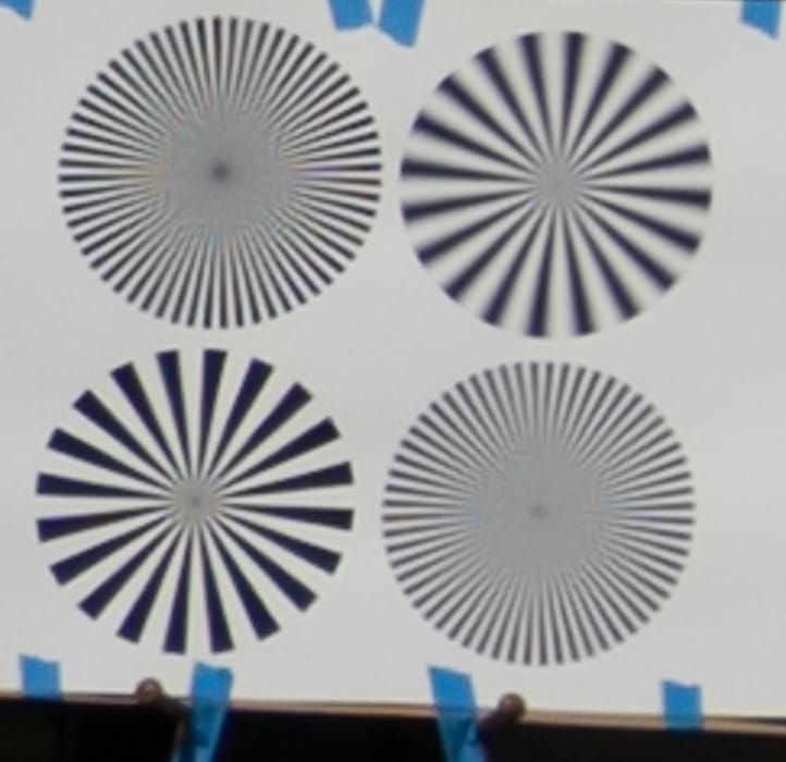
This lens has very little field tilt. The field is commendably flat. I see no astigmatism.

I’m going to redo the target for the next test. At present, I see no advantage to the sinusoidal Siemens Star for this test, but it may be different with a sensor with no AA filter.


The Last Word

← Sony 70-200/4@200mm on a9: tilt, field curvature, & astigmatism Fuji 110/2 on GFX, off-axis performance →

Comments

  1. Jack Hogan says

    September 6, 2017 at 1:53 am

    Jim, it won’t make a difference for the binary star, but did you gamma-encode the sinusoidal one before printing?

    Reply
    • JimK says

      September 6, 2017 at 7:37 am

      No.The print is linear. Bart suggested that a gamma-corrected star might be better for machine analysis, but I never followed up on that. I figured it should be linear for human viewing.

      Reply
      • Jack Hogan says

        September 6, 2017 at 8:16 am

        Having seen the results I don’t think it would make much of a difference in the final interpretation since it’s so qualitative – but it would make sense to me to feed the output device data encoded with the gamma it is expecting.

        On the other hand I would personally stick to linear where machine analysis is involved (e.g. FT/MTF).

        Reply
        • JimK says

          September 6, 2017 at 8:20 am

          When taking an image of the printed star and looking at it on the monitor in Lightroom, the eye sees a linear image, neglecting the slight contrast boost provided by the default Lr setting. Linear image captured by camera as linear raw, and gamma-corrected by Lr for the display, right? When the file is exported by Lr, it is gamma corrected for an sRGB display.

          Reply
          • Jack Hogan says

            September 7, 2017 at 12:50 am

            Right. I was thinking of when the sinusoidal star was printed, assuming it was generated in Matlab. But it would indeed be a small difference.

            Reply
            • JimK says

              September 7, 2017 at 7:41 am

              The print workflow is as follows: the star in generated in Matlab in linear space. It is written to a file in Adobe RGB (gammma 2.2), It is loaded into Ps, and tagged as an Adobe RGB file (Matlab doesn’t do the tagging). It is printed from Ps. Does that sound OK to you?

              Reply
              • Jack Hogan says

                September 7, 2017 at 10:28 am

                Since you apply the gamma 2.2 in Matlab it’s perfect!

                Reply

Leave a Reply Cancel reply

Your email address will not be published. Required fields are marked *

May 2025
S M T W T F S
 123
45678910
11121314151617
18192021222324
25262728293031
« Apr    

Articles

  • About
    • Patents and papers about color
    • Who am I?
  • How to…
    • Backing up photographic images
    • How to change email providers
    • How to shoot slanted edge images for me
  • Lens screening testing
    • Equipment and Software
    • Examples
      • Bad and OK 200-600 at 600
      • Excellent 180-400 zoom
      • Fair 14-30mm zoom
      • Good 100-200 mm MF zoom
      • Good 100-400 zoom
      • Good 100mm lens on P1 P45+
      • Good 120mm MF lens
      • Good 18mm FF lens
      • Good 24-105 mm FF lens
      • Good 24-70 FF zoom
      • Good 35 mm FF lens
      • Good 35-70 MF lens
      • Good 60 mm lens on IQ3-100
      • Good 63 mm MF lens
      • Good 65 mm FF lens
      • Good 85 mm FF lens
      • Good and bad 25mm FF lenses
      • Good zoom at 24 mm
      • Marginal 18mm lens
      • Marginal 35mm FF lens
      • Mildly problematic 55 mm FF lens
      • OK 16-35mm zoom
      • OK 60mm lens on P1 P45+
      • OK Sony 600mm f/4
      • Pretty good 16-35 FF zoom
      • Pretty good 90mm FF lens
      • Problematic 400 mm FF lens
      • Tilted 20 mm f/1.8 FF lens
      • Tilted 30 mm MF lens
      • Tilted 50 mm FF lens
      • Two 15mm FF lenses
    • Found a problem – now what?
    • Goals for this test
    • Minimum target distances
      • MFT
      • APS-C
      • Full frame
      • Small medium format
    • Printable Siemens Star targets
    • Target size on sensor
      • MFT
      • APS-C
      • Full frame
      • Small medium format
    • Test instructions — postproduction
    • Test instructions — reading the images
    • Test instructions – capture
    • Theory of the test
    • What’s wrong with conventional lens screening?
  • Previsualization heresy
  • Privacy Policy
  • Recommended photographic web sites
  • Using in-camera histograms for ETTR
    • Acknowledgments
    • Why ETTR?
    • Normal in-camera histograms
    • Image processing for in-camera histograms
    • Making the in-camera histogram closely represent the raw histogram
    • Shortcuts to UniWB
    • Preparing for monitor-based UniWB
    • A one-step UniWB procedure
    • The math behind the one-step method
    • Iteration using Newton’s Method

Category List

Recent Comments

  • bob lozano on The 16-Bit Fallacy: Why More Isn’t Always Better in Medium Format Cameras
  • JimK on Goldilocks and the three flashes
  • DC Wedding Photographer on Goldilocks and the three flashes
  • Wedding Photographer in DC on The 16-Bit Fallacy: Why More Isn’t Always Better in Medium Format Cameras
  • JimK on Fujifilm GFX 100S II precision
  • Renjie Zhu on Fujifilm GFX 100S II precision
  • JimK on Fuji 20-35/4 landscape field curvature at 23mm vs 23/4 GF
  • Ivo de Man on Fuji 20-35/4 landscape field curvature at 23mm vs 23/4 GF
  • JimK on Fuji 20-35/4 landscape field curvature at 23mm vs 23/4 GF
  • JimK on Fuji 20-35/4 landscape field curvature at 23mm vs 23/4 GF

Archives

Copyright © 2025 · Daily Dish Pro On Genesis Framework · WordPress · Log in

Unless otherwise noted, all images copyright Jim Kasson.