Most serious photographers, engineers, and scientists know about the inverse-square relationship of light intensity versus distance from a point source. Double the distance, and you get a quarter of the photon flux that passes through a given plane area normal to the direction of the light. Most engineers and scientists — but surprisingly, not most photographers — know that this only applies to point sources. For an infinite line source, luminous intensity falls off as distance, not distance squared. Move twice as far away, get half as much light. For an infinite plane source, luminous intensity doesn’t diminish with distance at all. Double the distance, get the same amount of light. A collimated source behaves the same way, but for different reasons.
A lot of photographers use light modifiers that try to provide a flat, diffuse, roughly circular source of illumination. Most soft boxes, all parabolic beauty dishes, most flatter beauty dishes, and even some LED panels are examples. They are often used close to the subject, so that the apparent angular size of the light, as seen by the subject, is large, making the light diffuse and the shadows soft. In that usage, the light is far from a point source. How does it diminish with distance?
There is a rule of thumb that you get close to inverse-square behavior if the distance from the subject to the diffuse lighting surface is greater than five times the diameter of the radiator. Some folks are more conservative and say it takes ten times the distance.
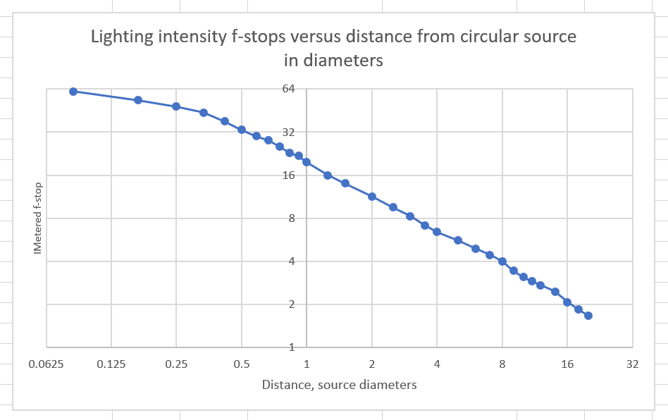
But how does the falloff behave when you’re closer than 5 diameters? I decided to find out. There are two ways that came to mind. The first was to write a simulation. But that would take a while (and cause me to think pretty hard), and there are always people who don’t believe the results of any simulation, so I turned to the second approach: set up a light and make a bunch of measurements. I set up a 12-inch parabolic beauty dish with a shower-cap diffuser on an Aputure 120D-II Bowens-mount light. I put new batteries in my trusty Minolta incident light meter, which has a hemispherical diffuser. I made a set of measurements at distances ranging from 0 to 240 inches away. I converted the distances in inches to diameters of the source by dividing by 12. I plotted the result with base 2 log-log axes.
Here it is:
Both linear and inverse-square responses result in straight lines on log-log plots. I plotted both:
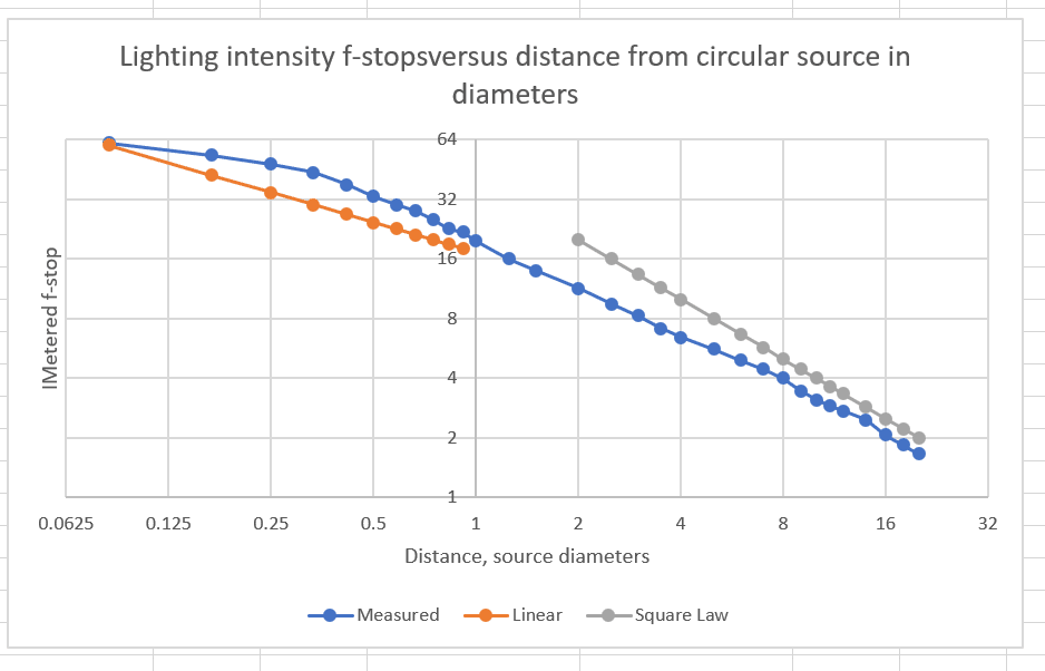
Slopes flatter than the orange line represent falloff that’s slower than linear. Slopes flatter than the blue line represent falloff that’s slower than inverse square. You can see that the falloff starts out slower than linear, and is about linear by the time you’re half a diameter away from the light. By the time you’re 8 times the diameter away from the light, the falloff slope is about inverse-square. Looks like the conservative 10x rule of thumb was pretty good, and the more liberal 5x one isn’t too far off.
There is a fudge that you sometimes see: say the inverse square law applies all the time, but call the distance the distance to the light source at the back of the light modifier. You can see right away that there’s a problem here: a long parabolic reflector is going to have a lot more distance added than a short beauty dish. If you compare the deep reflector to a LED-panel softbox like the Westcott ones, the disparity is even greater.
Nevertheless, I plunged ahead and added the diameter-and-a-quarter dish depth to the distances, and replotted the curve:
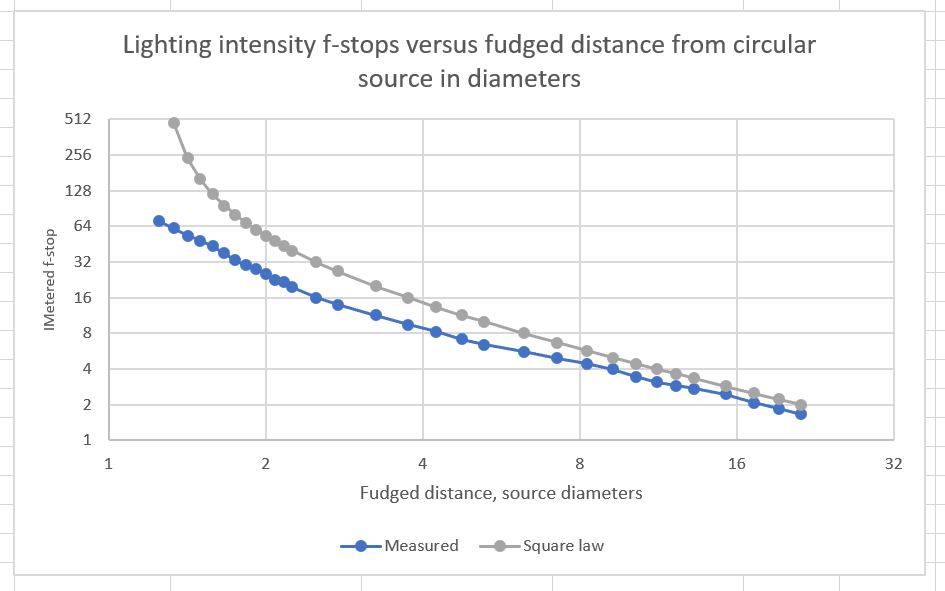
The agreement isn’t too bad until about the fudged distance is about 4 diameters (actual distance around 3 diameters), so the fudge is an improvement over just calling the whole thing inverse square. But things really fall apart when you get close to the radiator.
After I finished this post, I found this graph that summarizes a mathematical analysis of the issue:
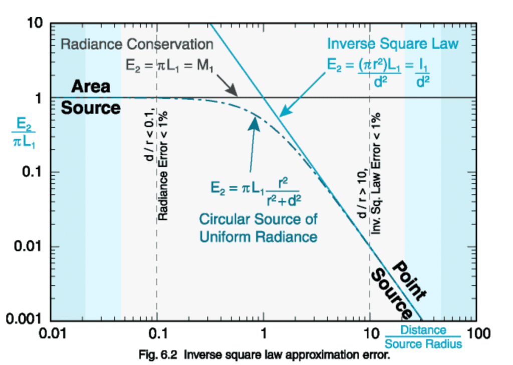
The x-axis is the ratio of distance to radius of the source, not diameter, which is what I used. So when the ratio is 10, the error is 1%. At that point the ratio of the distance to the diameter is 5, which must the the basis for the rule of thumb I mentioned above.
Nice article!
I would argue that a collimated light source falls off (or actually doesn’t) for exactly the same reason as an infinite plane source… no curvature of wavefronts so no geometrical spreading of energy… with collimation, the plane wavefronts are created from a discrete source.
With reflectors, I have always estimated the apparent distance of the point source to estimate fall-off. When I did wedding photography, I used a little portable, over-the-shoulder, reflector which placed the apparent position of the flash unit about 10 feet behind me and gave really even lighting over the depth of group shots.
If you look at it that way, you’re right.
That’s basically the “fudge” that I tested. It didn’t work well when the apparent size of the light source was large.
Re “rules of thumb”:
For most *photographic* purposes we can treat the falloff as 1/d^2 when (d/r) is > 3 (or so).
At that point the difference between 1/d^2 and 1/(r^2+d^2) is less than 1/6 EV.