• site home
  • blog home
  • galleries
  • contact
  • underwater
  • the bleeding edge

the last word

Photography meets digital computer technology. Photography wins -- most of the time.

You are here: Home / The Last Word / Mach banding

Mach banding

April 24, 2014 JimK 1 Comment

Inspired by the last three posts, I’m starting a series of posts on spatial considerations in color vision, which an emphasis on what’s important to photographers. We’ll get started today with an illustration:

Take good look at this image from a normal viewing distance:

machband

The bars are even steps along the grey axis in a linear RGB color space, so if you plotted the linear values as a graph with full scale being 1.0 and the column index increasing from left to right, here’s what you’d see:

mach actual

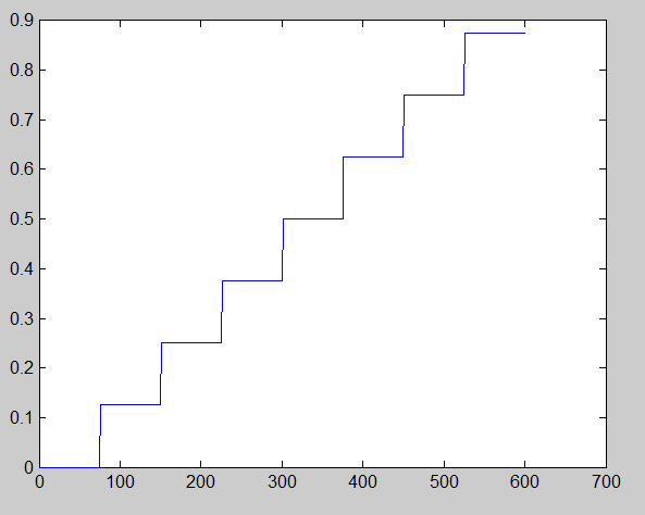
But that’s not what it looks like, is it? It looks more like the intensities go like this:

mach looks like

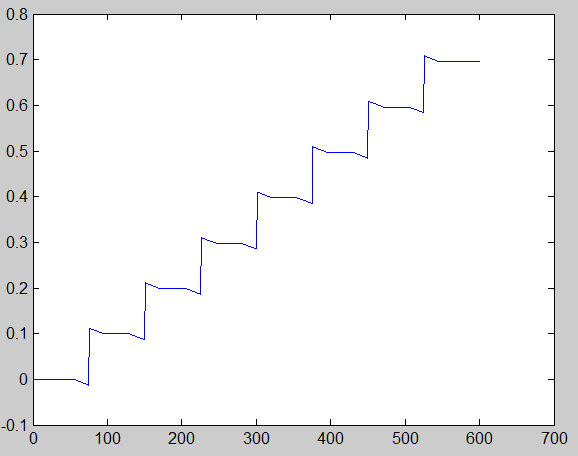
Get up real close to your screen and look at the step wedge above. You can still see the overshoot that’s not really there, right? Now back way up and look at it from across the room. Unless you’ve got a pretty big room, you can still see the phantom overshoots.

But if we take an image like this, which is just a smaller version of the step wedge, and you back up from it quite a ways, it looks like a smooth gradient:

machbandsm

The overshoots that aren’t really there are called Mach Bands, after Ernst Mach, who died about a hundred years ago, and also gave us the speed of sound as a unit of velocity measurement .

Mach bands are surprisingly robust. You can’t think them away by reminding yourself that they’re not real. They look the same if you rotate the step wedge by 90 degrees:

machbandv

Or some arbitrary angle:

machband45

The phenomenon is independent of color (but harder to see in the blue image, given the relative paucity of short (aka blue) cone cells):

machbandg

machbandr

machbandb

That’s our first lesson: the human vision system produces its internal definition of brightness by spatially differentiating light intensity for large features, and integrating light intensity for small features.

The Last Word

← Luminance and chromaticity vs spatial frequency, part 2 Looking for Mach Bands in chromaticity step wedges →

Comments

  1. ShowBlender says

    November 23, 2014 at 4:25 pm

    Neat! Mach Banding has practical applications in design, and more importantly, could also be attributed to some false diagnostics in medical imaging. I wrote a Mac app to help identify the issue with an image histogram to show the actual light properties vs perception. I’d like to know what you thought! Thanks for the article!

    Reply

Leave a Reply Cancel reply

Your email address will not be published. Required fields are marked *

May 2025
S M T W T F S
 123
45678910
11121314151617
18192021222324
25262728293031
« Apr    

Articles

  • About
    • Patents and papers about color
    • Who am I?
  • How to…
    • Backing up photographic images
    • How to change email providers
    • How to shoot slanted edge images for me
  • Lens screening testing
    • Equipment and Software
    • Examples
      • Bad and OK 200-600 at 600
      • Excellent 180-400 zoom
      • Fair 14-30mm zoom
      • Good 100-200 mm MF zoom
      • Good 100-400 zoom
      • Good 100mm lens on P1 P45+
      • Good 120mm MF lens
      • Good 18mm FF lens
      • Good 24-105 mm FF lens
      • Good 24-70 FF zoom
      • Good 35 mm FF lens
      • Good 35-70 MF lens
      • Good 60 mm lens on IQ3-100
      • Good 63 mm MF lens
      • Good 65 mm FF lens
      • Good 85 mm FF lens
      • Good and bad 25mm FF lenses
      • Good zoom at 24 mm
      • Marginal 18mm lens
      • Marginal 35mm FF lens
      • Mildly problematic 55 mm FF lens
      • OK 16-35mm zoom
      • OK 60mm lens on P1 P45+
      • OK Sony 600mm f/4
      • Pretty good 16-35 FF zoom
      • Pretty good 90mm FF lens
      • Problematic 400 mm FF lens
      • Tilted 20 mm f/1.8 FF lens
      • Tilted 30 mm MF lens
      • Tilted 50 mm FF lens
      • Two 15mm FF lenses
    • Found a problem – now what?
    • Goals for this test
    • Minimum target distances
      • MFT
      • APS-C
      • Full frame
      • Small medium format
    • Printable Siemens Star targets
    • Target size on sensor
      • MFT
      • APS-C
      • Full frame
      • Small medium format
    • Test instructions — postproduction
    • Test instructions — reading the images
    • Test instructions – capture
    • Theory of the test
    • What’s wrong with conventional lens screening?
  • Previsualization heresy
  • Privacy Policy
  • Recommended photographic web sites
  • Using in-camera histograms for ETTR
    • Acknowledgments
    • Why ETTR?
    • Normal in-camera histograms
    • Image processing for in-camera histograms
    • Making the in-camera histogram closely represent the raw histogram
    • Shortcuts to UniWB
    • Preparing for monitor-based UniWB
    • A one-step UniWB procedure
    • The math behind the one-step method
    • Iteration using Newton’s Method

Category List

Recent Comments

  • bob lozano on The 16-Bit Fallacy: Why More Isn’t Always Better in Medium Format Cameras
  • JimK on Goldilocks and the three flashes
  • DC Wedding Photographer on Goldilocks and the three flashes
  • Wedding Photographer in DC on The 16-Bit Fallacy: Why More Isn’t Always Better in Medium Format Cameras
  • JimK on Fujifilm GFX 100S II precision
  • Renjie Zhu on Fujifilm GFX 100S II precision
  • JimK on Fuji 20-35/4 landscape field curvature at 23mm vs 23/4 GF
  • Ivo de Man on Fuji 20-35/4 landscape field curvature at 23mm vs 23/4 GF
  • JimK on Fuji 20-35/4 landscape field curvature at 23mm vs 23/4 GF
  • JimK on Fuji 20-35/4 landscape field curvature at 23mm vs 23/4 GF

Archives

Copyright © 2025 · Daily Dish Pro On Genesis Framework · WordPress · Log in

Unless otherwise noted, all images copyright Jim Kasson.