• site home
  • blog home
  • galleries
  • contact
  • underwater
  • the bleeding edge

the last word

Photography meets digital computer technology. Photography wins -- most of the time.

You are here: Home / The Last Word / Manipulating MTF50 hyperfocal distances

Manipulating MTF50 hyperfocal distances

June 14, 2016 JimK 2 Comments

This is a continuation of a report on new ways to look at depth of field. The series starts here:

A new way to look at depth of field

For the past few posts, I’ve been developing the concept of a hyperfocal distance based on the allowable degradation of image resolution as measured by MTF50. There are two convenient properties of hyperfocal distance as calculated using the conventional circle of confusion (CoC) methods.

  • If you focus the lens at infinity, the allowable near limit of sharpness occurs at the hyperfocal distance.
  • If you focus the lens at the hyperfocal distance, the allowable near limit of sharpness occurs at half the hyperfocal distance.

Wouldn’t it be nice if both those things applied to the new MTF50-based hyperfocal distance? It turns out they do, perhaps not exactly, but darned close.

If we focus our top-notch 55 mm lens at almost infinity, here’s what we get:

HFD 55 infinity

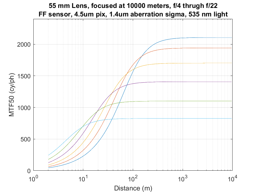
Now, let’s say that we want the hyperfocal distance (HFD) for 90% of the resolution available at infinity when the lens is focused there. If, for each aperture, we drop down on the right side of the graphs to 90% of the MTF50 value where the line hits the end of the graph, and trace that value back to the left on the graph until we encounter the line for that aperture, we get the hyperfocal distance for that sharpness tolerance and aperture.

If we run a set of curves with the lens focused to those hyperfocal distances, we get this:

55mmHFDMTFratio p9

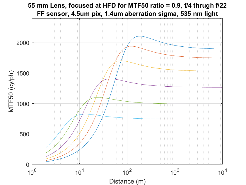
The peaks are at the hyperfocal distances for each stop (no surprise there; that’s where we focused the lens). The amount of sharpness reduction at infinity in each case is the reduction we saw when we graphically found the HFDs. You’re going to have to trust me on this last one, since the distance scale is compressed, but the place where the sharpness nearer than the HFD falls to the value at infinity is half of the HFD.

Here are two more graphs for lower tolerance ratios:

55mmHFDMTFratio p8

55mmHFDMTFratio p6

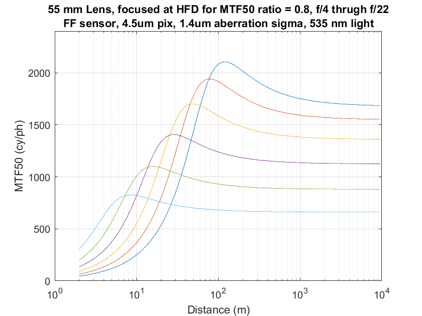
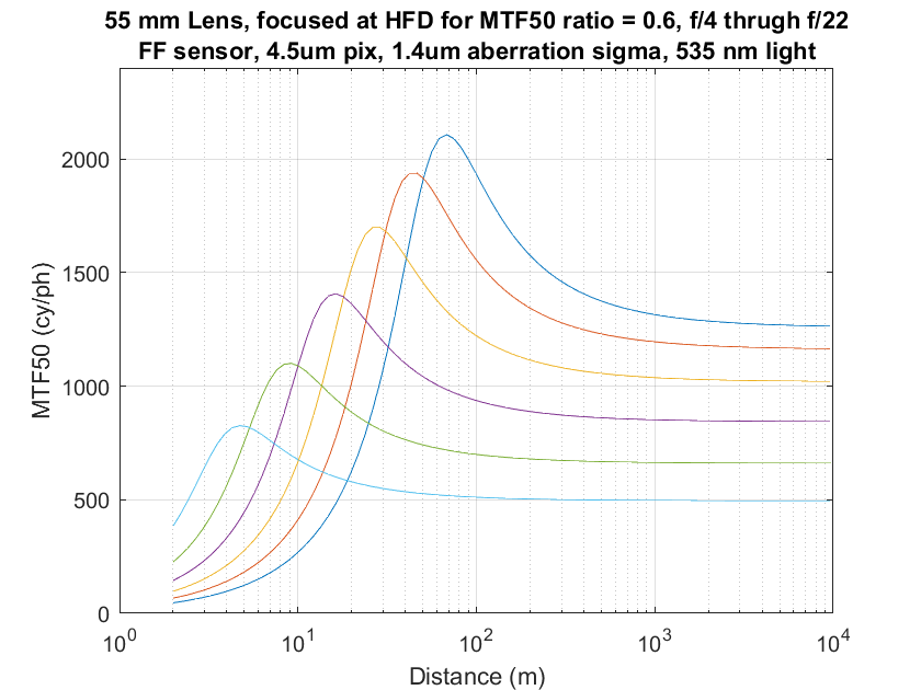
The same thing happens. I’m not sure exactly why this is true, but it’s very convenient. [Edit:  The surprise to me was that relationship survives even after all the additional sources of blurring other than defocus.  Thinking about it now, it makes sense, since the model for all those is that they are insensitive to defocusing, and thus affect the near and the far points equally.]

The Last Word

← Calculating hyperfocal distances using absolute MTF50 values Obtaining absolute MTF50 hyperfocal distances →

Comments

  1. CarVac says

    June 14, 2016 at 2:30 pm

    So the real relation would be that the sharpness at infinity is equal to sharpness at 1/2 the focus distance, regardless of whether or not you’ve done hyperfocal distance or gone for the bokeh.

    And that makes sense, actually. In image space, they’re roughly the same distance away from the focal point, so they’ll be blurred equally (as a first order approximation).

    Thin lens equation: 1/s1 + 1/s2 = 1/f

    When f = 50mm and s1 is 5000 mm, you get s2 = 50.5050…mm.

    When f = 50mm and s1 is 2500 mm, you get s2 = 51.0204…mm.

    When f = 50mm and s1 is infinity, you get s2 = 50mm.

    They’re about equidistant from the focal plane.

    Reply
    • Jim says

      June 14, 2016 at 3:42 pm

      Right. The surprise to me was that relationship survives even after all the additional sources of blurring other than defocus. Thinking about it now, it makes sense, since the model for all those is that they are insensitive to defocusing, and thus affect the near and the far points equally. I think I’ll go back and add that.

      Jim

      Reply

Leave a Reply Cancel reply

Your email address will not be published. Required fields are marked *

May 2025
S M T W T F S
 123
45678910
11121314151617
18192021222324
25262728293031
« Apr    

Articles

  • About
    • Patents and papers about color
    • Who am I?
  • How to…
    • Backing up photographic images
    • How to change email providers
    • How to shoot slanted edge images for me
  • Lens screening testing
    • Equipment and Software
    • Examples
      • Bad and OK 200-600 at 600
      • Excellent 180-400 zoom
      • Fair 14-30mm zoom
      • Good 100-200 mm MF zoom
      • Good 100-400 zoom
      • Good 100mm lens on P1 P45+
      • Good 120mm MF lens
      • Good 18mm FF lens
      • Good 24-105 mm FF lens
      • Good 24-70 FF zoom
      • Good 35 mm FF lens
      • Good 35-70 MF lens
      • Good 60 mm lens on IQ3-100
      • Good 63 mm MF lens
      • Good 65 mm FF lens
      • Good 85 mm FF lens
      • Good and bad 25mm FF lenses
      • Good zoom at 24 mm
      • Marginal 18mm lens
      • Marginal 35mm FF lens
      • Mildly problematic 55 mm FF lens
      • OK 16-35mm zoom
      • OK 60mm lens on P1 P45+
      • OK Sony 600mm f/4
      • Pretty good 16-35 FF zoom
      • Pretty good 90mm FF lens
      • Problematic 400 mm FF lens
      • Tilted 20 mm f/1.8 FF lens
      • Tilted 30 mm MF lens
      • Tilted 50 mm FF lens
      • Two 15mm FF lenses
    • Found a problem – now what?
    • Goals for this test
    • Minimum target distances
      • MFT
      • APS-C
      • Full frame
      • Small medium format
    • Printable Siemens Star targets
    • Target size on sensor
      • MFT
      • APS-C
      • Full frame
      • Small medium format
    • Test instructions — postproduction
    • Test instructions — reading the images
    • Test instructions – capture
    • Theory of the test
    • What’s wrong with conventional lens screening?
  • Previsualization heresy
  • Privacy Policy
  • Recommended photographic web sites
  • Using in-camera histograms for ETTR
    • Acknowledgments
    • Why ETTR?
    • Normal in-camera histograms
    • Image processing for in-camera histograms
    • Making the in-camera histogram closely represent the raw histogram
    • Shortcuts to UniWB
    • Preparing for monitor-based UniWB
    • A one-step UniWB procedure
    • The math behind the one-step method
    • Iteration using Newton’s Method

Category List

Recent Comments

  • JimK on Goldilocks and the three flashes
  • DC Wedding Photographer on Goldilocks and the three flashes
  • Wedding Photographer in DC on The 16-Bit Fallacy: Why More Isn’t Always Better in Medium Format Cameras
  • JimK on Fujifilm GFX 100S II precision
  • Renjie Zhu on Fujifilm GFX 100S II precision
  • JimK on Fuji 20-35/4 landscape field curvature at 23mm vs 23/4 GF
  • Ivo de Man on Fuji 20-35/4 landscape field curvature at 23mm vs 23/4 GF
  • JimK on Fuji 20-35/4 landscape field curvature at 23mm vs 23/4 GF
  • JimK on Fuji 20-35/4 landscape field curvature at 23mm vs 23/4 GF
  • Ivo de Man on Fuji 20-35/4 landscape field curvature at 23mm vs 23/4 GF

Archives

Copyright © 2025 · Daily Dish Pro On Genesis Framework · WordPress · Log in

Unless otherwise noted, all images copyright Jim Kasson.